Averaged Control

PDF version | Download Matlab Code | Download Scilab Code | GITHUB

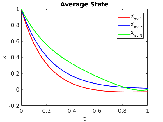
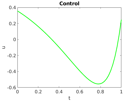
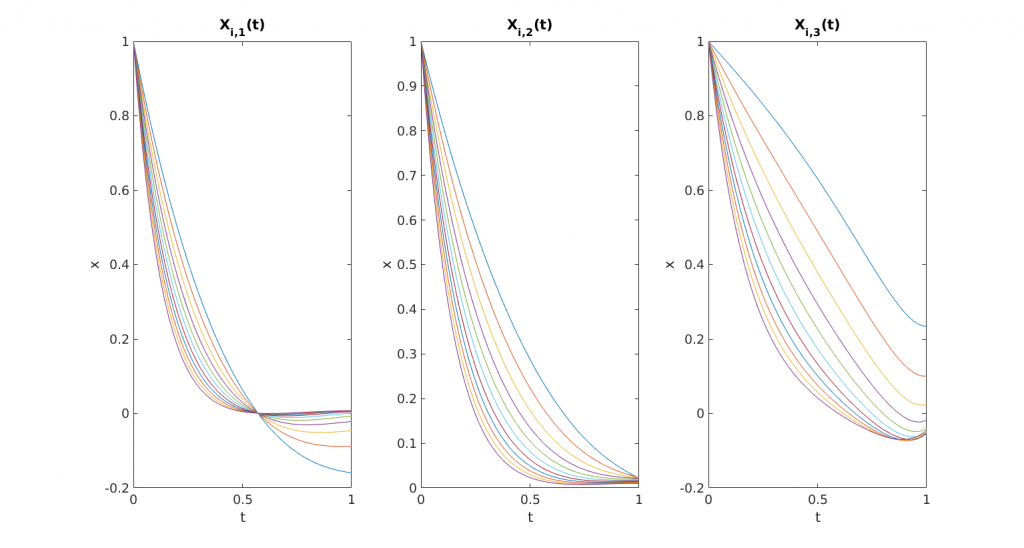
In this work, we address the optimal control of parameter-dependent systems. We introduce the notion of averaged control in which the quantity of interest is the average of the states with respect to the parameter family $\mathcal{K}= \left\{ \nu_i \in \mathbb{R}, \enspace 1\leq i \leq K \right\}$. More precisely, we are interested in solving the minimization problem

$$\begin{equation} \label{eq:costFunctional}
\min _{u \in L^2(0,T)} \mathcal{J}\left( u\right) = \min _{u \in L^2(0,T)} \frac{1}{2} \left[ \frac{1}{K} \sum_{\nu \in \mathcal{K}} x \left( T, \nu \right) – \bar{x} \right]^2 + \frac{\beta}{2} \int_0^T u^2 \mathrm{d}t, \quad \beta \in \mathbb{R}^+
\end{equation}$$

where $\mathcal{U}_{ad}$ is the space of admissible controls and $\bar{x}$ the average state target. The optimization problem (\ref{eq:costFunctional}) is subject to the finite dimensional linear control system

\begin{align} \label{eq:primalODE}
\left\{
\begin{array}{ll}
x^\prime \left( t \right) = A \left( \nu \right) x \left( t \right) + B \left( \nu \right) u \left( t \right), \quad 0 < t Algorithm 1 Optimal control with Conjugate Gradient Method

Require: $A\left( \nu \right)$, $B\left( \nu \right)$, $x^0$, $u^{\left(0\right)}$, $\beta$, $T$, $\bar{x}$, $tol$

1. $n \gets 0 $
2. compute $\bar{y} \left( T \right)$
3. $b \gets \Lambda^*\left( \bar{x} – \bar{y} \left( T \right) \right)$
4. $z \gets \Lambda u$
5. $g \gets \Lambda^*z + \beta u – b$
6. $h \gets ||g||^2_{L^2\left(\left[0,T\right]\right)}$
7. $h_a \gets h$
8. $r \gets -g$
9. While $||r||_{L^2\left(\left[0,T\right]\right)} > tol $ do
10.     $z \gets \Lambda r$
11.     $w \gets \Lambda^*z + \beta r$
12.     $\alpha \gets \frac{h}{\left(r,w\right)_{L^2\left(\left[0,T\right]\right)}}$
13.     $u \gets u + \alpha r$
14.     $g \gets g + \alpha w$
15.     $h_a \gets h$
16.     $h \gets ||g||^2_{L^2\left(\left[0,T\right]\right)}$
17.     $\gamma \gets \frac{h}{h_a}$
18.     $r \gets -g + \gamma r$
19.     $n \gets n + 1$

Bibliography

[1] E. Zuazua (2014) Averaged Control. Automatica, 50 (12), p. 3077-3087.

Authors: Víctor Hernández-Santamaría, José Vicente Lorenzo, Enrique Zuazua

March, 2018