1. Numerical experiments
Consider the one dimensional linear Vlasov-Fokker-Planck (VPFP) as following.
\begin{equation}
\begin{cases}
\delta\pt_tf + \sigma_1v\delta\pt_x f – \frac{\sigma_2}{\epsilon} \delta\pt_x\phi\delta\pt_v f =\frac{\sigma_3}{\epsilon}\delta\pt_v\ (v f +\delta\pt_vf\ ), \qd t>0, x\in[0,2\pi], v\in \mathbb{R}, \label{eq: VPFP}\\
f(0, x,v,z) = f_0(x,v,z), \qd z\in [a,b].
\end{cases}
\end{equation}
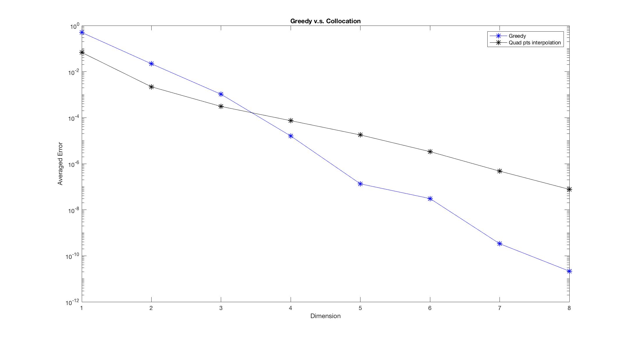
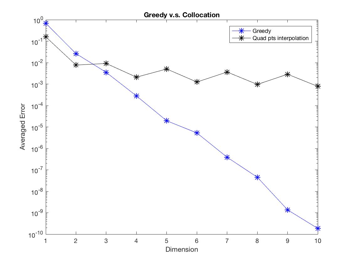
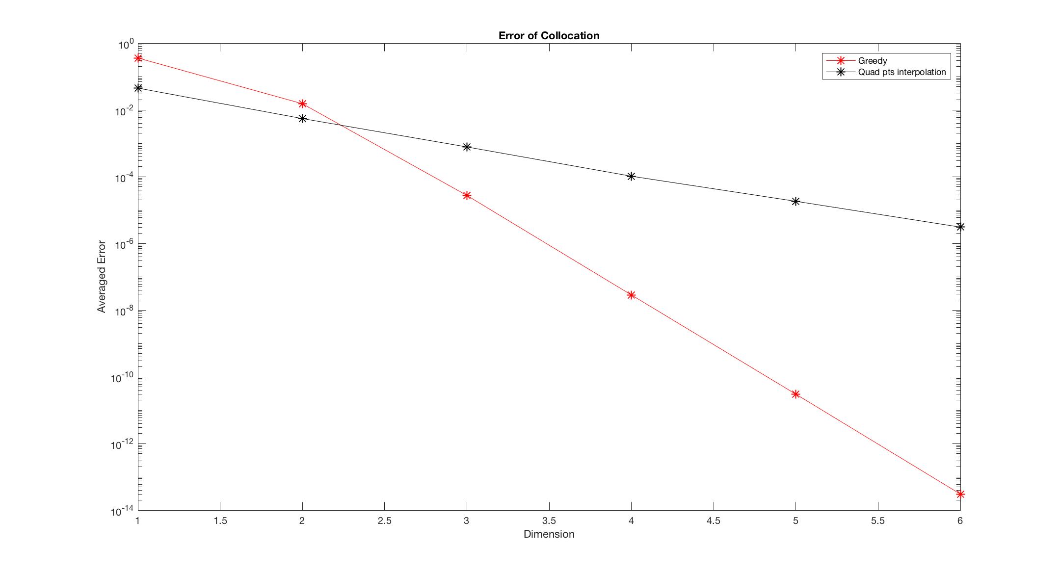
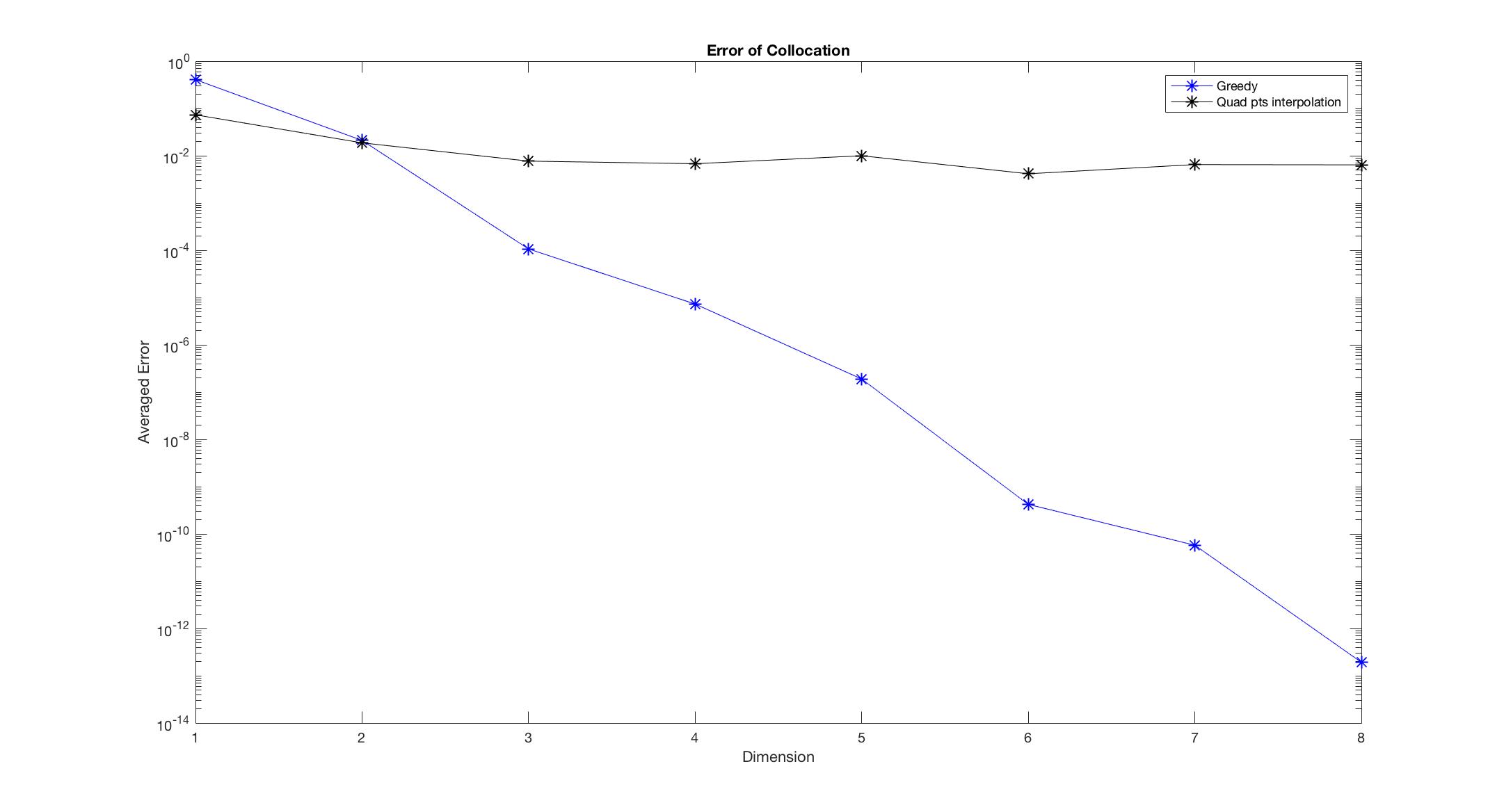
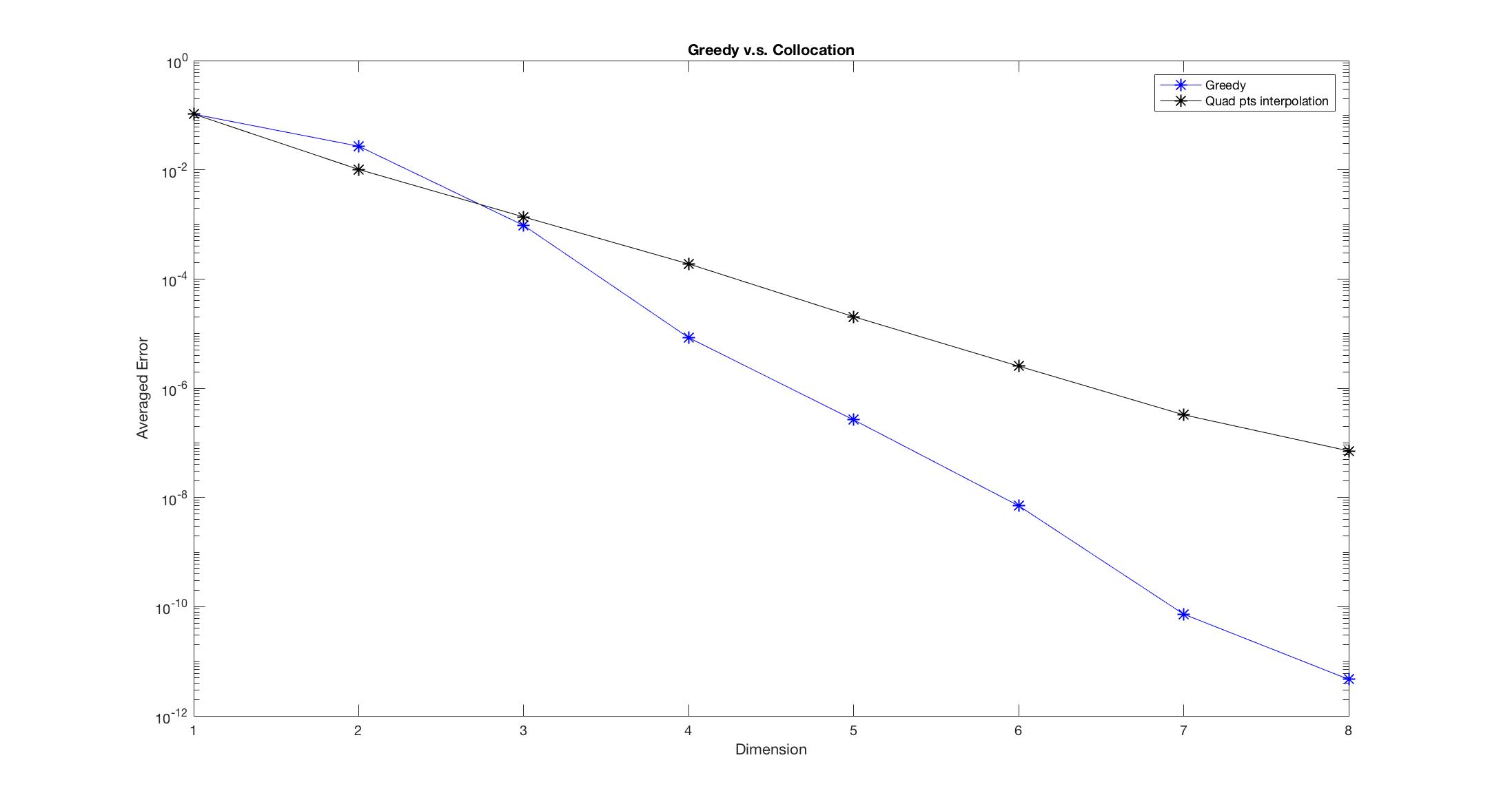
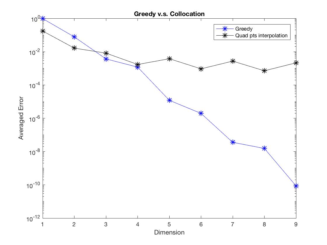
In the numerical experiments, we compare the results from the greedy algorithm with the results from the polynomial interpolation of the quadrature points. we set $\epsilon = 1, T = 0.5$ for all examples. More specifically, we set $$\bf{$\text{error} = \sum_{i=1}^{50}\int{ {( \hat{f}(T, x, v, z_i) – f(T, x,v,z_i) )}^2} dxdv$, where $\hat{f}(T, x,v,z_i)$ $$ is the approximation solution obtained from either method, $f(T, x,v,z_i)$ is the exact solution. $z_i$ is uniformly chosen from $[a,b]$. ${\bf{Dimension}}$ refers to the number of snap shots.
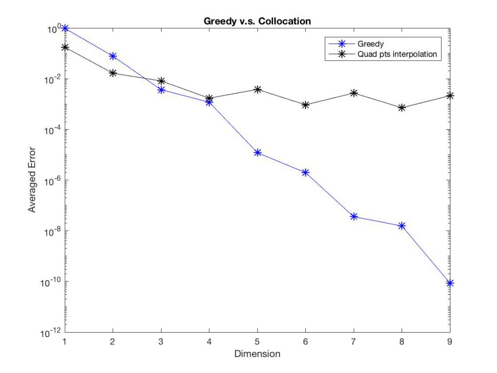
Observe Figure 1-6, we found that the Greedy algorithm converges to the solution faster than the other method. Especially, when there is discontinuity, the polynomial interpolation doesn’t converge as dimension increases, however, the Greedy algorithm still converges and almost keeps the same convergent rate.
Algorithm 1.1. The algorithm for the polynomial interpolation:
For Dimension $= n$, $\{\alpha_i\}_{i=1}^n$ is the n roots of $n$-th order Legendre polynomial, and let
\begin{equation}
z_i ^*= \frac{b-a}{2}\alpha_i + \frac{a+b}{2}, \qd 1\leq i \leq n.\label{}
\end{equation}
\begin{equation}
f_i = f(T, x,v, z_i ^*) \text{ be the exact solution at time T}.\label{}
\end{equation}
Then by Lagrange interpolation,
\begin{align}
\hat{f}(T,x,v,z) = \sum_{i=1}^n l_i(z)f_i,\qd l_i = \prod_{j\neq i} \frac{z-z_j ^*}{z_i ^* – z_j ^*}
\end{align}
1.1 Linear VFP with parametric initial data
In the first experiment, we consider the case where the parameter $z\in[1,5]$ only involved in the initial data,
\begin{equation}
\sigma_1 = \sigma_2 = \sigma_3 = 1, \delta \pt_x\phi = \cos(x), \qd
\end{equation}
Figure 1: \begin{equation} f_0(x,v,z) = \frac{1}{\sqrt{2\pi}} (2+\frac{\sin(x)}{z}) \text{exp} (-\frac{\lv \abs{v+\cos(x) + \frac{z}{10} }^2}{2} ).\end{equation}
Figure 2: \begin{equation} f_0(x,v,z) =\left\{
\begin{array}{rl}
\frac{1}{\sqrt{2\pi}} (2+\frac{\sin(x)}{z}) \text{exp} (-\frac{\lv \abs{v+\cos(x) + \frac{z}{10} }^2}{2} ),\qd z<3\\
\frac{1}{\sqrt{2\pi}} (2+\frac{\sin(x)}{z}) \text{exp} (-\frac{\lv \abs{v+\cos(x) + \frac{z+1}{10} }^2}{2} ),\qd z\geq3.
\end{array}
\right.\end{equation}
Algorithm 1.2. The algorithm for PDE with only parameter in initial data:
Offline:
Step 1: Set $N = \{z_i: z_i = i\delta_z, \delta_z = \frac{b-a}{N_z}, i = 0,1, \dots, N_z\}$, we set $N_z = 100$ in this case.
\begin{equation}
z_1^* = \text{argmax}_{z\in N} \abs{ \abs{ f_0(x,v,z) } } ^2,
\end{equation}
where $\abs{ \abs{ f }}^2 = \int f^2\,dxdv$.
Step 2: After obtaining $z_i^*, f_i = f_0(x,v,z_i^*)$, $i =1, \dots, n-1$,
\begin{equation}
z_n^* = \text{argmax}_{z\in N\backslash\{z_i^*\}_{i=1}^{n-1} } \abs{ \abs{ f_0(x,v,z) – P^{n-1} f_0(x,v,z) }}^2,
\end{equation}
where $P^{n-1} f_0$ is the projection onto the subspace spanned by $f_1, \dots, f_{n-1}$
Step 3: Stops when
\begin{equation}
\max_{z\in N\backslash\{z_i^*\}_{i=1}^{n-1} } \abs{ \abs{ f_0(x,v,z) – P^{n-1} f_0(x,v,z)}}^2 \leq \epsilon
\end{equation}
Online: After we obtained the snap shots $\{z_i^*\}_{i=1}^n$,
Step 1: Orthogonalize $\{f_i\}_{i=1}^n$, and calculate the corresponding $\{ f^T_i = f(T,x,v,z_i) \}_{i=1}^n$.
Step 2: for any given $z$, one can approximate $f(T, x,v,z)$ by
\begin{equation}
a_i = \langle f_0(x,v,z), f_i\rangle, \qd \hat{f}(x,v, z) = \sum_{i = 1}^na_if^T_i.
\end{equation}
1.2 Linear parametric VFP with deterministic initial data
In the second experiment, we consider the case where the parameter $z\in[1,5]$ only involved in the PDE,
\begin{equation}
& f_0(x,v,z) = \frac{1}{\sqrt{2\pi}} ( 2+\sin(x) ) \text{exp} ( -\frac{|v+\cos(x)|^2}{2} ),
\end{equation}
Figure 3: \begin{equation}\sigma_1 = 1+\frac{1.5}{z},\qd \sigma_2 = \sigma_3 = 1+5e^{\frac{1}{z}}, \qd\delta_x\phi = \cos(x)+\frac{z}{10};\end{equation}
Figure 4: \begin{equation}\sigma_1 = 1+\frac{1.5}{z},\qd \sigma_2 = \sigma_3 = 1+5e^{\frac{1}{z}}, \qd\delta_x\phi =\left\{
\begin{array}{rl}
& \cos(x)+\frac{z}{10},\qd z<3\\
&\cos(x)+\frac{z+1}{10},\qd z\geq3
\end{array}
\right.
\end{equation}
Algorithm 1.3. The algorithm for PDE with only parameters in PDE:
Offline: Set $N = \{z_i: z_i = i\delta_z, \delta_z = \frac{b-a}{N_z}, i = 0,1, \dots, N_z\}$, we set $N_z = 100$ in this case.
Step 1: choose $z_1^* = argmax_{z\in N} \abs{ \abs{ (\sigma_1,\sigma_2,\sigma_3\)}}^2$.
Step 2: After obtaining $z_i^*, f_i = f(T,x,v,z_i^*)$, $i =1, \dots, n-1$,
\begin{equation}z_n^* = argmax_{z\in N\backslash\{z_i^*\}_{i=1}^{n-1}} [ \min_{\hat{f} = \sum a_if_i, \sum a_i = 1} \abs{ \abs{ \delta_t\hat{f} + \underbrace{ \sigma_1(z)v\delta_x \hat{f} – \frac{\sigma_2(z)}{\epsilon} \delta_x\phi\delta_v \hat{f} – \frac{\sigma_3(z)}{\epsilon}\delta_v ( v \hat{f} + \delta_v\hat{f} ) }_{A(z)\hat{f} } } }^2 ],
\label{linear z_star}
\end{equation}
Step 3: Stops when the above maximum residual smaller than $\epsilon$.
Online: After we obtained the snap shots $\{z_i\}_{i=1}^n$, and the corresponding $f_i = f(T, x,v,z_i)$,
\begin{equation}
\hat{f} = \argmin_{\hat{f} = \sum a_if_i, \sum a_i = 1} \abs{ \abs{ \delta_t\hat{f} + \underbrace{\sigma_1(z)v\delta_x \hat{f} – \frac{\sigma_2(z)}{\epsilon} \delta_x\phi\delta_v \hat{f} – \frac{\sigma_3(z)}{\epsilon}\delta_v (v \hat{f} +\delta_v\hat{f} ) }_{A(z)\hat{f} } } }^2
\end{equation}
1.3 Linear parametric VFP with parametric initial data
In the third experiment, we consider the case where the parameter $z\in[1,5]$ involved in both the initial data and the PDE, \begin{equation}\sigma_1 = 1+\frac{1.5}{z},\qd \sigma_2 = \sigma_3 = 1+5e^{\frac{1}{z}},\qd f_0(x,v,z) = \frac{1}{\sqrt{2\pi}}(2+\frac{\sin(x)}{z}) \text{exp}(-\frac{|v+\delta_x\phi|^2}{2}).\end{equation}
Figure 5: \begin{equation}\delta_x\phi = \cos(x) + \frac{z}{10},\qd \text{for }t\geq 0,\end{equation}
Figure 6: \begin{equation}\delta_x\phi =\left\{\begin{array}{rl}& \cos(x)+\frac{z}{10},\qd z<3\\&\cos(x)+\frac{z+1}{10},\qd z\geq3\end{array}\right.\qd \text{for }t\geq 0.\end{equation}
Algorithm 1.4. The algorithm for PDE with parameters in PDE and initial data:
Offline: Set $N = \{z_i: z_i = i\delta_z, \delta_z = \frac{b-a}{N_z}, i = 0,1, \dots, N_z\}$, we set $N_z = 10000$ in this case.
Step 1: Using Algorithm 1.4 to obtain 50 snap shots out of $N$ to form a new set $N^*$.
Step 2: Using Algorithm 1.3 to get snap shot $\{ z_i^* \}_{i=1}^n.$
Online: Same as Algorithm 1.3.
Remark 1.5. In the experiments, the exact solution $f(T,x,v,z)$ refers to the numerical solution to VFP, that is, $f(T,x,v,z)$ is a $N_x\times N_v$ dimensional vector obtained by the following scheme
\begin{equation}
\frac{f^{n+1}_{i,j} – f^n_{i,j}}{\delta_t} +\sigma_1 (v\delta_xf)^n_{i,j} = \frac{\sigma_3}{\epsilon}P(f^{n+1}_{i,j})
\end{equation}
where $P(f)$ is the discretization of $\delta_v (M\delta_v (\frac{f}{M}))$, $M = \frac{1}{\sqrt{2\pi}}e^{-\frac{\abs{v+\frac{\sigma_2}{\sigma_3}\delta_x\phi}^2}{2}}$.
Remark 1.6. For the matlab coding, the algorithm for the examples is in the “graph.m” file of the folder “eq1”, “eq2”, “eq3” respectively. You can change the coefficients in “sig_1”, “sig_2”, “sig_3”, and the electric field in “fcn_phi_x”, and initial data in “fcn_phi_x_0”, “fcn_rho_0”.
P.S. Remember to change the path of other functions at the beginning of “graph.m”.