1. Problem formulation
Let $\Omega\subset \mathbb R^d$ be an open and bounded Lipschitz Domain and consider the parameter dependent parabolic equation with Dirichlet boundary conditions
\begin{equation}\label{heat_intro}
\begin{cases}
y_{t}-\textnormal{div}(a(x,\nu)\nabla y) +c\, y=\chi_\omega u \quad &\text{in } Q=\Omega\times(0,T), \\
y=0 \quad &\text{on } \Sigma=\partial\Omega\times(0,T), \\
y(x,0)=y^0(x) \quad&\text{in } \Omega,
\end{cases}
\end{equation}
where $y=y(x,t;\nu)$ is the state, $u=u(x,t)$ is a control function and $y_0$ is given initial datum.
In (1), $a(x,\nu)$ is a scalar $L^\infty(\Omega)$ coefficient depending on some parameter $\nu$ and $c=c(x)\in L^\infty(\Omega)$ is given. To abridge the notation, we will denote $a_\nu=a(x,\nu)$.
Now, consider the following associated optimal control problem
\begin{equation}\label{min_evo_intro}
\min_{u\in L^2(0,T;L^2(\omega))} \, J^T(u)=\frac{1}{2}\int_{0}^T|u(t)|^2_{L^2(\omega)}+\frac{\beta}{2}\int_{0}^T\|y(t)-y_d\|^2_{L^2(\Omega)},
\end{equation}
where $y$ is the solution to (1), $y_d\in L^2(\Omega)$ is a desired observation and $\beta>0$ is given.
It is classical to prove (see e.g., [3]) that the minimization problem (2) has a unique optimal solution that hereinafter we denote by $(u^T,y^T)$. Moreover, the optimal control is given by
\begin{equation*}\label{opt_evo}
u^T=-\chi_\omega p^T
\end{equation*}
where $q^T$ can be found from the solution $(y^T,p^T)$ of the optimality system
\begin{equation}\label{opt_sys_evolution}
\begin{cases}
y^T_t-\textnormal{div}(a_\nu \nabla y^T) +c\, y^T =-\chi_\omega p^T, \quad &\text{in } Q, \\
-p_t^T-\textnormal{div}(a_\nu \nabla p^T) +c\, p^T=\beta\,(y^T-y_d), \quad &\text{in } Q, \\
y^T=q^T=0, \quad &\text{on } \Sigma, \\
y^T(x,0)=y^0, \quad q^T(x,T)=0, \quad &\text{in } \Omega.
\end{cases}
\end{equation}
In this work, we use a combination of (weak) greedy methods and the so-called turnpike property to determine the most relevant values of a parameter-space providing the best possible approximation of the set of parameter dependent optimal controls.
Firstly, we will use the turnpike property to reduce the problem of computing the time-dependent optimal controls $u^T$ by computing asymptotic simplifications.
To this end, we begin by considering the stationary version of the state equation
\begin{equation}\label{steady_state}
\begin{cases}
-\textnormal{div}(a_\nu \nabla y)+c \, y=\chi_\omega u \quad &\text{in } \Omega, \\
y=0 \quad &\text{on } \partial \Omega. \\
\end{cases}
\end{equation}
Now, consider the corresponding minimization problem
\begin{equation}\label{min_steady_intro}
\min_{u\in L^2(\omega)} \, J(u)=\frac{1}{2}|u|^2_{L^2(\omega)}+\frac{\beta}{2}\|y-y_d\|^2_{L^2(\Omega)}.
\end{equation}
As before, one can prove that, since $J$ is strictly convex, continuous and coercive, the minimization problem (5) has a unique optimal solution $(\bar u, \bar y)$, where the optimal control is characterized by
\begin{equation*}
\bar u=-\chi_\omega \bar p,
\end{equation*}
and $(\bar y, \bar p)$ solve the optimality system
\begin{equation}\label{opt_sys_steady}
\begin{cases}
-\textnormal{div}(a_\nu \nabla \bar y) +c\, \bar y=-\chi_\omega \bar p, \quad &\text{in } \Omega, \\
-\textnormal{div}(a_\nu \nabla \bar p) +c\, \bar p=\beta\,(\bar y-y_d), \quad &\text{in } \Omega, \\
\bar y=\bar p=0, \quad &\text{on } \partial \Omega. \\
\end{cases}
\end{equation}
A natural question that arises in this context is to which extent the long horizon optimal controls and states $(u^T(t),y^T(t))$ approach the steady ones $(\bar u,\bar y)$ as $T\to +\infty$. According to [4], we have the following result:
Theorem 1.1
Let us consider the control problem (2) and let $(u^T,y^T)$ be the optimal control and state. Then, there exists $\mu>0$ such that
\begin{equation}\label{conv_exponential}
\|y^T(t)-\bar y\|_{L^2(\Omega)}+\|u^T(t)-\bar u\|_{L^2(\Omega)} \leq K\left( e^{-\mu t}+e^{-\mu(T-t)}\right), \quad \forall t\in [0,T],
\end{equation}
where $(\bar u,\bar y)$ is the optimal control and state corresponding to (6).
This means that we have exponential convergence of the finite horizon control problems to their steady state version as $T$ tends to infinity.
Thanks to Theorem 1.1, we can now focus our attention on the steady system (4). We begin by assuming the following hypotheses:
\begin{enumerate}
\item[\textbf{H1}] The parameter $\nu$ ranges within a compact set $\mathcal K \subseteq \mathbb{R}^d$.
\item[\textbf{H2}] The coefficient functions $a_\nu$ are bounded functions satisfying uniform coercive and boundedness estimates:
\begin{equation*}
\begin{aligned}
& 0 < a_1\leq \norm{a_\nu}_{L^\infty(\Omega)} \leq a_2,\quad &\nu \in K.
\label{UEA}
\end{aligned}
\end{equation*}
In addition, $a_\nu$ depend on $\nu$ in an analytic manner .
\end{enumerate}
[/latex]
Then, the main idea is to propose a methodology to determine an optimal selection of a finite number of realizations of the parameter $\nu$ so that all controls, for all possible values of $\nu$, are optimally approximated. More precisely, the problem can be formulated as follows:
<strong>Problem 1.2</strong>
Let us consider the set of controls verifying (5) for each possible value $\nu \in \mathcal K$. That is,
\begin{equation}
\overline{\mathcal U}=\left\{\bar u_\nu : \nu\in \mathcal K\right\}.
\end{equation}
This control set is compact in $L^2(\omega)$. </p>
<p>Given $\varepsilon>0$, we seek to determine a family of parameters $\{\nu_1,\ldots,\nu_n\}$ in $\mathcal K$, whose cardinality $n$ depends on $\varepsilon$, so that the corresponding controls, denoted by $u_{\nu_1},\ldots,u_{\nu_n}$ are such that for every $\nu\in \mathcal K$, there exists $u_\nu^\star\in \textnormal{span}\{u_{\nu_1},\ldots,u_{\nu_n}\}$ such that
[latex]
\begin{equation*}
\|u_\nu^\star-\bar u_\nu\|\leq \varepsilon.
\end{equation*}
2. Greedy optimal control for elliptic problems
2.1. Preliminaries on (weak) greedy algorithms
In this section, we present a short introduction about linear approximation theory of parametric problems based on (weak) greedy algorithms. For a more detailed read, we refer, for instance, to [1, 2]. In general, the goal is to approximate a compact set $\mathcal K$ in a Banach space $X$ by a sequence of finite dimensional subspaces $V_n$ of dimension $n$.
The algorithm reads as follows.
The algorithm produces a finite dimensional space $V_n$ that approximates the set $\mathcal K$ within precision $\varepsilon$.
The best choice of an approximating space $V_n$ is the one producing the smallest approximation error. This smallest error for a compact set $\mathcal K$ is called the Kolmogorov $n$-width of $\mathcal K$, and is defined as
\begin{equation*}
d_n(\mathcal K):=\inf_{\dim Y=n} \sup_{x\in \mathcal K} \, \inf_{y\in Y} \|{x-y}\|_X\,.
\end{equation*}
It measures how well $\mathcal K$ can be approximated by a subspace in $X$ of a fixed dimension $n$.
Algorithm 1: Weak greedy algorithm
initialize: fix $\gamma\in (0,1]$ and a tolerance parameter $\varepsilon>0$;
- In the first step, choose $x_1\in\mathcal K$ such that
- At the general step, having found $x_1,\ldots,x_n$ denote
- repeat
- choose $x_{n+1}$ such that
- until$\sigma_n(\mathcal K)<\varepsilon$;
2.2. Definition of the residual
The main goals of this work is to apply the greedy approach to the family of parameter dependent steady state optimal control problems
\begin{equation}\label{min_P}
\left(\mathcal{P}\right) \ \ \ \ \ \ \ \min_{u\in L^2(\omega)} \left\{ J_\nu( u)\right\},
\end{equation}
where $J$ is the cost functional given by
\begin{equation*}
\label{J}
J_\nu( u) = \frac{1}{2} |{u}|_{L^2(\omega)}^2 \ + \ \frac{1}{2} \norm{y_\nu(u)-y^d}^2_{L^2(\Omega)},
\end{equation*}
while $y_\nu(u)$ is the solution to (4).
Essential for an effective application of a greedy algorithm is the construction of a residual by which one can estimate the distance between two (possible unknowns) controls by some easily computable quantity.
In this way, we introduce the residual operator as
\begin{equation}
\label{res}
\begin{aligned}
R_\nu(p,y):=\left(
\begin{matrix} L_\nu y+ \chi_\omega p\\
L_\nu p- \beta\left( y - y^d\right) \\
\end{matrix}\right).
\end{aligned}
\end{equation}
The residual $R_\nu(p,y)$ introduced in the previous subsection enable us to construct a weak greedy algorithm for an effective construction of an approximating linear space of the control manifold $\overline \lU$. The precise description of the the algorithm is given below
We can summarize the obtained results in the following theorem
Theorem 2.1
The proposed greedy algorithm provides the following estimates on the approximate control and approximate optimal state
\begin{equation*}
\begin{aligned}
& \bullet\quad \norm{u_\nu^\star - \bar u_\nu}_{L^2(\Omega)} \leq \varepsilon, \\
& \bullet \quad \norm{ y_\nu^\star - \bar y_\nu}_{\Hj\Omega}
\leq \left({\varepsilon \over \alpha_1 }\right)
\end{aligned}
\end{equation*}
3. Numerical experiments
We present here two numerical examples where the greedy approach is applied. To illustrate the procedure, we consider the two dimensional domain $\Omega=(0,1)^2$. We use the elementary finite difference (FD) method. We will approximate the elliptic operator $\mathcal A=-\textnormal{div}(a_\nu\nabla \,\cdot)$ with homogeneous Dirichlet boundary conditions, by using the standard 5-point discretization.
3.1. Greedy test # 1
Let us consider a coefficient $a_\nu$ of the form
\begin{equation}\label{coef_exp1}
a_\nu(x)=1+\nu(x_1^2+x_2^2)
\end{equation}
where we assume that
\begin{equation}\label{range_exp1}
\nu\in [1,10]=\mathcal K.
\end{equation}
In this way, we can readily verify that $a_\nu$ satisfies H1 and H2.
On the other hand, we take the coefficient $c$ as
\begin{equation*}
c(x)=\sin(\pi x_1)\sin(\pi x_2).
\end{equation*}
which clearly fulfills the condition $c\geq 0$. For the optimal control problem, we set the parameter $\beta=10^4$ while the desired target is the $x_2$-independent function
\begin{equation*}
y^d(x)=\sin(2\pi x_1).
\end{equation*}
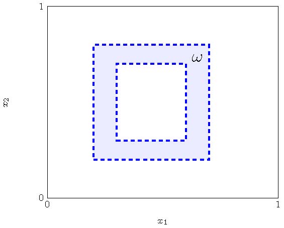
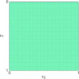
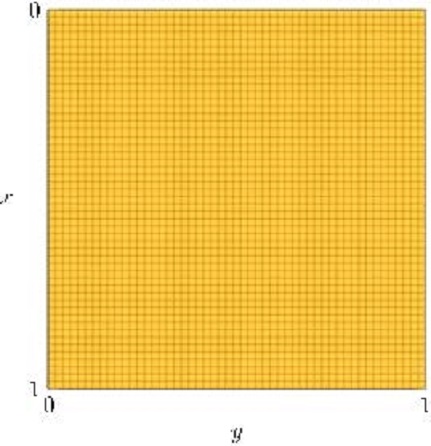
We take $\omega$ as the region $(0.2,0.5)\times(0,5,0.9)\cup(0.5,0.9)\times(0.1,0.9)$ in the $x_1x_2$-plane (see Figure 2.B).
Algorithm 2: Greedy control algorithm - offline part
Initialize: Fix the approximation error $\varepsilon>0$.
- STEP 1: (discretisation)
- Choose a finite subset $\tilde{\mathcal K}$ such that
$\forall{\nu} \in \mathcal K \quad dist(\nu, \tilde{\mathcal K}) <\delta,$- for $\delta>0$ a discretization constant.
- STEP 2: (Choosing $\nu_1$)
- Check the inequality
\begin{equation}\label{1st_stop} \max_{\tilde{\nu} \in \tilde{\mathcal K}} \|\beta y^{d}_{\nu}\|_{H^{-1}\Omega} <\frac{\varepsilon} 2.\; \end{equation} [/latex] </div> </li> <li>If it is satisfied, stop the algorithm. Otherwise, choose the first parameter value as <div align="center"> [latex] \begin{equation}\label{first_sel} \nu_1 \in arg\max_{\tilde{\nu} \in \tilde{\mathcal K}} \{ \|y^{d}_{\nu}\|_{H^{-1}(\Omega)}\}.; \end{equation}- and find corresponding optimal primal and dual states $\bar y_1, \bar p_1$;
- STEP 3: (Choosing $\nu_{j+1}$)
- Having chosen $\nu_1, \ldots, \nu_j$ calculate $R_{\tilde \nu}(\bar p_j, 0)$ and $R_{\tilde \nu}(0, \bar y_j)$ for each $\tilde \nu \in \tilde{\mathcal K}$.
- Check the approximation criteria
\begin{equation} \label{stop_crit} \max_{\tilde\nu \in \tilde{\mathcal K}} ||\inf_{( p, y) \in (\overline{\mathcal P}_j, \overline{\mathcal Y}_j)} R_{\tilde \nu}(p, y) ||_{H^{-1}(\Omega)} < \frac{\varepsilon}2. \end{equation} [/latex] </div> </li> <li>If the inequality is satisfied, stop the algorithm. Otherwise, determine the next parameter value as <div align="center"> [latex] \begin{equation} \label{step_j} \nu_{j+1}\in arg\max_{\tilde \nu \in \tilde{\mathcal K}} || \inf_{( p, y) \in (\overline{\mathcal P}_j, \overline{\mathcal Y}_j)} R_{\tilde \nu}(p, y) ||_{H^{-1}(\Omega)}, \end{equation}- Find the corresponding optimal primal and dual states $\bar y_{j+1}, \bar p_{j+1}$ and repeat Step 3.
Since the functional $J_\nu$ is quadratic and coercive, a standard conjugate gradient (CG) algorithm is a simple choice to solve the minimization problem (5). For a given $\nu\in\mathcal K$ one can directly solve the minimization problem (10). The average time for computing the corresponding control up to a given tolerance of $10^{-8}$ using the CG is around six seconds.
Hypotheses H1 and H2 allow us to implement a naive approach for approximating the parameterized control set $\bar{\mathcal U}(\mathcal K)$. This approach consists in discretizing the parameter set in a very fine mesh, that we denote it by $\tilde{\mathcal K}$, and then computing the corresponding control for each parameter in this finite-dimensional set.
Let us take $\tilde{\mathcal K}$ as the uniform discretization of the interval (13) in $k=100$ values. Then, the naive approach amounts to solve 100 different times the minimization problem (10). The whole process takes around $600$ seconds.
We apply the greedy procedure described in Algorithm 2 over the set $\tilde{\mathcal K}$ and choosing a precision of $\varepsilon=0.005$. The algorithm stops after seven iterations selecting 7 (out of 100) parameter values. The time needed to finish the offline part of the greedy algorithm takes 476 seconds.
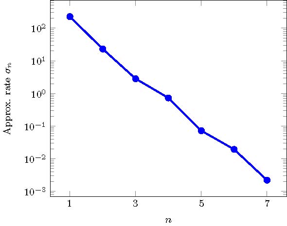
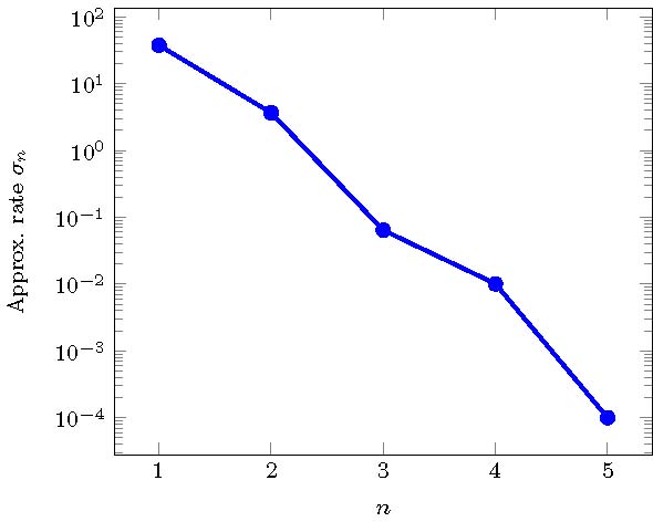
\begin{equation*} \sigma_n(\tilde{\mathcal K})=\max_{\nu\in\tilde{\mathcal K}}\dist \Big((\bar p_\nu,\bar y_\nu),(\bar {\mathcal P}_n,\bar {\mathcal Y}_n)\Big). \end{equation*} Such plot suggests an exponential decay of the approximation rate $\sigma_n$, which is in accordance with the greedy theory.
Once the offline part is completed, we can construct (approximate) optimal controls by choosing a suitable combination of the optimal states $\bar p_{\nu_i}$.
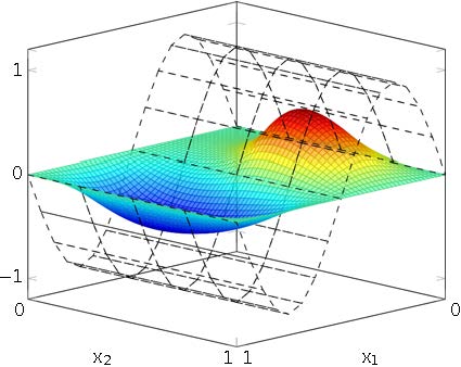
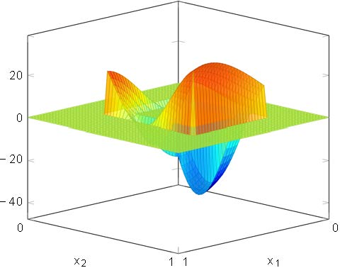
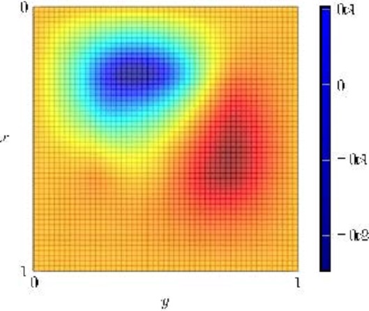
In Figure 2, we plot the approximation of the real control with the greedy algorithm for $\nu=\sqrt 2$. The approximated control is nearly identical to the obtained by minimizing directly functional (5) for the associated value $\nu=\sqrt{2}$. In fact, one can obtain for this particular experiment that
\begin{equation*}
\|\bar{u}_{\sqrt 2}- u_{\sqrt 2}^\star\|_{L^2(\Omega)}\approx 4.61\times 10^{-5}.
\end{equation*}
In spite of obtaining almost the same solution, the convergence of conjugate gradient method takes 5.4 s compared to 0.488 s in the online greedy part. This fact also shows the computational efficiency of the proposed algorithm.
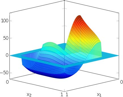
In Figure 3.A, we plot the solution to (4) using the approximated control $u_{\sqrt{2}}^\star$. As for the control, we can compute the difference between the real optimal state against the approximate optimal state $\bar y^\star_{\sqrt 2}$. In this particular test, we obtain the following estimate
\begin{equation*}
\|\bar{y}_{\sqrt 2}- y_{\sqrt 2}^\star\|_{L^2(\Omega)}\approx 7.14\times 10^{-7}.
\end{equation*}

3.2. Greedy test # 2
Here, we present a series of experiments for the case when the potential fulfills $c(x)\leq 0$. This will be of particular interest in the discussion of the following section.
We consider again the coefficient (12) and the parameter $\nu$ within the range (13), as in the previous test. For this particular case, we choose a constant function $c$ and the desired target as follows
\begin{equation*}
c(x)\equiv-37 \quad{\text{and}}\quad y^d(x)=\sin(\pi x_1)
\end{equation*}
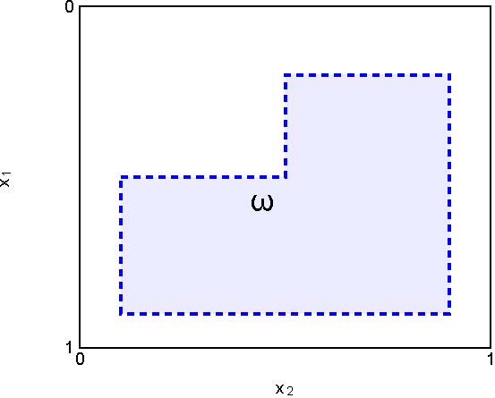
We will use as a control region the shape depicted in figure 4. For this particular test, the average time for computing the optimal control for different values of $\nu$ is around nine seconds. Implementing the naive approach for the refined mesh $\tilde{\mathcal K}$ implies that at least 900 seconds are needed to finish this process.
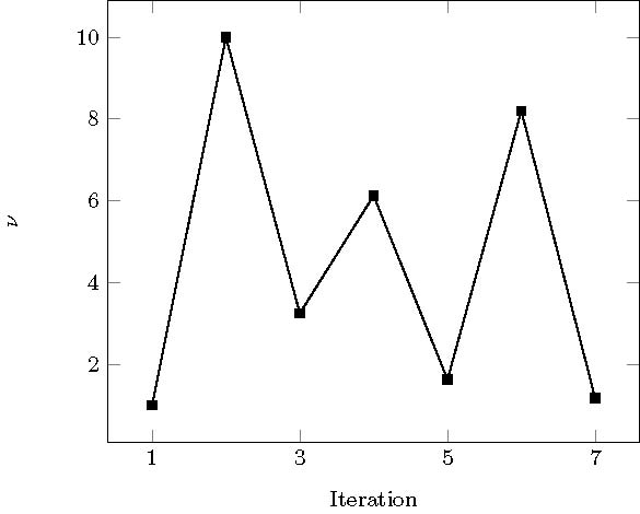
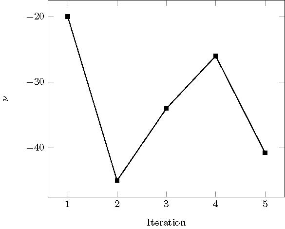
Using our computational tool, we choose again the approximation tolerance $\varepsilon=0.005$. The greedy algorithm stops after nine iterations. We present in figure 5a the selected parameters in the order they were chosen by the program. The elapsed time for completing the offline process is 678 seconds.
In Figure 6 we plot the approximation of the optimal control obtained by the greedy method for a chosen value of $\nu=7/5$, while in Figure 7 we show corresponding controlled state and a comparison with the target $y^d$. For this particular test, the elapsed time to compute the online control is 0.406 seconds while the convergence of the CG to compute the optimal control takes 15.9 seconds. The approximation error with respect to the real control is
\begin{equation*}
\|\bar u_{7/5}- u^\star_{7/5}\|_{L^2(\Omega)}\approx 1.46\times 10^{-4},
\end{equation*}
while the approximation error for the state using the real and approximated control is
\begin{equation*}
\|\bar y_{7/5}- y^\star_{7/5}\|_{L^2(\Omega)}\approx 4.78\times 10^{-5}.
\end{equation*}
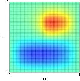
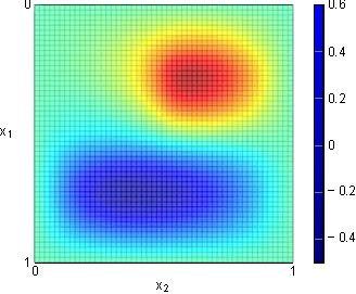
In Figure 7, we observe that the approximation to the desired target $y^d$ is (to a certain extent) better than the one we obtain in greedy test #1. This is because the chosen $y^d$ does not change sign in the domain $\Omega$ (cf. Figure 3.B).
where $y$ is solution to the parabolic problem
\begin{equation}\label{evo_turn_6}
\begin{cases}
y_t-\div(a_\nu \nabla y)+c\, y=1_\omega u, \quad &\text{in } \Omega\times(0,T), \\
y=0, \quad &\text{on } \partial \Omega\times(0,T), \\
y(x,0)=y^0(x), \quad &\text{in } \Omega.
\end{cases}
\end{equation}
Here, we present a series of experiments related to the (approximated) optimal steady controls in Sections 3.1 and 3.2. We use them to control the corresponding evolution equation and test their efficiency. We will differentiate two main cases to be studied.
The case $c(x)\geq 0$
In addition to the parameters already set in the greedy test #1 (see Section 3.1), let us take
\begin{itemize}
\item $T=3$,
\item $y^0(x)\equiv 0$.
\end{itemize}
In this stage, we are going to use the optimal control $\bar u^\star_{\sqrt 2}$ as a time-independent control for system (18). More precisely, we take
\begin{equation}\label{control_exp51}
u(x,t)=\bar u^\star_{\sqrt 2}(x) \quad\text{for }t\in (0,T).
\end{equation}
By plugging such control into equation (18), we obtain the controlled solution displayed in Figure 8. We see that this control steers $y$ away from the initial condition at time $t=0$ and reaches in a short amount of time a region near the optimal steady state $\bar y^\star_{\sqrt{2}}$ (cf. Figure 8.C).
For this experiment, the efficiency of the time-independent control is closely related to the fact that $c(x)\geq 0$. In particular, the conditions on the coefficients $a_\nu$ and $c$ allow to prove that the uncontrolled system (18) is exponentially stable regardless of the initial datum.
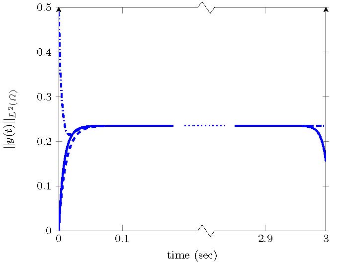
In Figure 9, we illustrate the efficiency of the steady control by plotting different curves representing the time evolution of the $L^2$-norm of $y$ solution to (18) with different initial datums and taking (19) as a control. To compare, we have computed the time-dependent solution $y^T(t)$ associated to the optimal control $u^T(t)$, obtained by minimizing (17), for the given parameter $\nu=\sqrt{2}$ and $y_0(x)=0$.
.
The case $c(x)< 0$
Let us take the parameters and results in the greedy test #2 shown in Section 3.2 together with $y_0(x)=0$ and $T=3$. As before, we can put the (approximated) steady control $\bar u^\star_{7/5}(x)$ in system (18) and test its performance. Recall that we have chosen $c(x)\equiv -37$. We show in Figure 10 the solution to the evolution problem using the steady control $\bar u^\star_{7/5}$. We see that in this case, the steady control lacks to stabilize the system around the steady state shown in figure 10.
In Figure 11, we present further experiments where we illustrate that for some initial data, the controlled solution $y$ grows in exponential manner. In fact, only for $y_0(x)=\bar y^\star_{7/5}$ and a sufficiently small neighborhood of this initial datum, the steady control is effective to control the underlying system.
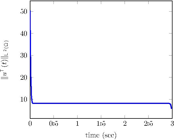
For this particular case, to see the turnpike property it is necessary to compute the solution to the time-dependent minimization problem (18). We show in Figure 12, the time evolution of the optimal controlled state and control and, as expected, we can see the asymptotic simplification towards the state and control for most of the time horizon. However, we can also see that the control makes a large effort at the beginning of the temporal interval to move the system to this steady state.
Unlike the case $c(x)\geq 0$, there might be some coefficients $c(x)<0$ such that steady controls, and in particular the approximated controls derived from the greedy approach, are not enough to control the evolution system.
Bibliography
[1] A. Cohen and R. DeVore Approximation of high-dimensional parametric PDEs. Acta Numerica, 24, (2015), 1--159.
[2] R. DeVore, (2005) The Theoretical Foundation of Reduced Basis Methods. preprint.
[3] J.-L Lions. Optimal control of systems governed by partial differential equations. Springer-Verlag, 1971.
[4] A. Porretta and E. Zuazua. Long time versus steady state optimal control. SIAM Journal on Control and Optimization, 51, 6 (2013), 4242-4273.
