Optimal Control of the Poisson Equation with OpenFOAM

PDF version | Download Openfoam Code… |

In this tutorial, we show how to use the C++ library OpenFOAM (Open Field Operation and Manipulation) in order to solve control problems for partial differential equations (PDE).

OpenFOAM is a free open source toolbox that allows the user to code customized solvers for Continuum Mechanics, with special attention to the field of Computational Fluid Dynamics. One can either use one of the multiple solvers already programmed for steady-state, transient or multiphase problems in fluid mechanics, or code his own solver depending on particular needs.

In this work, we will solve the optimal control problem

\begin{equation} \label{eq:CostFunctional}
\min _{u \in L^2 \left( \Omega \right)} \mathcal{J}\left( u\right) = \min _{u \in L^2 \left( \Omega \right)} \frac{1}{2} \int_{\Omega} \left( y – y_d \right) ^2 \mathrm{d} \Omega + \frac{\beta}{2} \int_{\Omega} u ^2 \mathrm{d} \Omega,
\end{equation}

where $u$ is the control variable, $y$ the state variable and $y_d$ a target function. The minimization problem is subject to the elliptic partial differential equation

\begin{align}
-\Delta y & = f + u && \mathrm{in} \enspace \Omega \label{eq:PoissonEq}, \\
\end{align}
\begin{align}
y & = 0 && \mathrm{on} \enspace \Gamma \label{eq:PoissonBC}.
\end{align}

We use some classical gradient descent methods based on the adjoint methodology, namely the steepest descent and conjugate gradient methods. The corresponding adjoint system for \ref{eq:PoissonEq} writes as,

\begin{align}
– \Delta \lambda & = y – y_d && \mathrm{in} \enspace \Omega, \label{eq:PoissonAdjointEq} \\
\end{align}
\begin{align}
\lambda & = 0 \ && \mathrm{on} \enspace \Gamma. \label{eq:PoissonAdjointBC}
\end{align}

In the steepest descent gradient method, we compute the directional derivative of the cost function in \ref{eq:CostFunctional},

\begin{equation}
J^\prime \left( u \right) \delta u = \int_{\Omega} \left( \lambda + \beta u \right) \delta u \mathrm{d} \Omega,
\end{equation}

where $\lambda$ is solution to the elliptic problem in \ref{eq:PoissonAdjointEq}, and use the gradient to update the control variable as

\begin{equation}
u^{\left( n + 1 \right)} = u^{\left( n \right)} – \gamma \left( \lambda^{\left( n \right)} + \beta u^{\left( n \right)} \right),
\end{equation}

for some value of $\gamma$.

One of the main advantages of OpenFOAM is its friendly syntax to describe PDE, as can be seen in the lines 10 and 13 in the code below.

// Initialize L2 norm of control update
scalar pL2 = 10*tol;
 
// Get the volume of mesh cells
scalarField volField = mesh.V();
 
while (runTime.loop() && ::sqrt(pL2) > tol)
{
    // Solve primal equation
    solve(fvm::laplacian(k, y) + u);
 
    // Solve ajoint equation
    solve(fvm::laplacian(k, lambda) + y - yd);
 
    // Update control
    p = lambda + beta*u;
    u = u - gamma*p;
 
    // Control update norm
    pL2 = ::sqrt(gSum(volField*p.internalField()*p.internalField()));
 
    // Compute cost function
    J = 0.5*gSum(volField*(Foam::pow(y.internalField()-yd.internalField(),2) \
	    + beta*Foam::pow(u.internalField(),2)));
 
    // Display information
    Info << "Iteration " << runTime.timeName() << " - " \
	    << "Cost value " << J << " - " \
	    << "Control variation L2 norm " << ::sqrt( pL2 ) << endl;
 
    // Save current iteration results
    runTime.write();
}

In order to improve the convergence to the optimal control, the conjugate gradient method is applied also to the problem. First, the state variable must be separated in two terms as

\begin{equation}
y = y_u + y_{f},
\end{equation}

where $y_u$ solves the state equation with zero Dirichlet boundary conditions,

\begin{align}
-\Delta y_u & = u && \mathrm{in} \enspace \Omega \label{eq:PoissonEqu}, \\
\end{align}
\begin{align}
y_u & = 0 && \mathrm{on} \enspace \Gamma \label{eq:PoissonBCu},
\end{align}

and $y_{f}$ is the control-free solution to the state equation,

\begin{align}
-\Delta y_{f} & = f && \mathrm{in} \enspace \Omega \label{eq:PoissonEq0}, \\
\end{align}
\begin{align}
y_{f} & = 0 && \mathrm{on} \enspace \Gamma \label{eq:PoissonBC0}.
\end{align}

Now, using the above separation of the state variable, one part depending on the control and the other part on a known source term, the cost functional in \ref{eq:CostFunctional} can be expressed as

\begin{equation} \label{eq:CostFunctionalcg}
J \left( u \right) = \frac{1}{2} \left( y_u + y_f – y_d, y_u + y_f – y_d \right)_{L^2\left( \Omega \right)} + \frac{\beta}{2} \left( u , u \right) _{L^2\left( \Omega \right)}.
\end{equation}

We define a linear operator $\Lambda: L^2\left( \Omega \right) \rightarrow L^2\left( \Omega \right)$ that takes a control $u$ and returns the solution to problem \ref{eq:PoissonEqu}-\ref{eq:PoissonBCu}, so that $y_u = \Lambda u$. We introduce as well its adjoint operator $\Lambda^*: L^2\left( \Omega \right) \rightarrow L^2\left( \Omega \right)$ that takes the source term in \ref{eq:PoissonAdjointEq} and solves the Poisson equation, so that $\lambda = \Lambda^* \left( y – y_d \right)$.

The directional derivative of the functional \ref{eq:CostFunctionalcg} then reads as

\begin{equation}
J^\prime\left( u \right) \delta u = \left( \underbrace{ \left( \Lambda^* \Lambda + \beta I \right)}_{A_{cg}} u – \underbrace{ \Lambda^* \left( y_d – y_f \right)}_{b_{cg}}, \delta u \right) _{L^2\left( \Omega \right)}.
\end{equation}

After having identified $A_{cg}$ and $b_{cg}$ we can use the conjugate gradient method to reach the optimal control faster.

Algorithm 1 Optimal control with Conjugate Gradient Method

Require: $y_D$, $u^{\left(0\right)}$, $\beta$, $y_d$, $tol$

$n \gets 0 $
compute the control-free solution, $y_f$
$b \gets \Lambda^*\left( y_d – y_f \right)$
$z \gets \Lambda u$
$g \gets \Lambda^*z + \beta u – b$
$h \gets ||g||^2_{L^2\left(\left[0,T\right]\right)}$
$h_a \gets h$
$r \gets -g$
While $||r||_{L^2\left(\left[0,T\right]\right)} > tol $ do
$z \gets \Lambda r$
$w \gets \Lambda^*z + \beta r$
$\alpha \gets \frac{h}{\left(r,w\right)_{L^2\left(\left[0,T\right]\right)}}$
$u \gets u + \alpha r$
$g \gets g + \alpha w$
$h_a \gets h$
$h \gets ||g||^2_{L^2\left(\left[0,T\right]\right)}$
$\gamma \gets \frac{h}{h_a}$
$r \gets -g + \gamma r$
$n \gets n + 1$

// Compute b: right-hand side of Ax = b
solve(fvm::laplacian(k, y));
solve(fvm::laplacian(k, lambda) + yd - y);
volScalarField b = lambda;
 
// Compute A*f0
// Primal equation
solve(fvm::laplacian(k, y0) + u);
// Adjoint equation
solve(fvm::laplacian(k, lambda) + y0);
 
// Compute g0: initial gradient
volScalarField g = lambda + beta*u - b;
scalar gL2 = gSum( volField * g.internalField() * g.internalField() );
scalar gL2a = 0;
 
// Compute initial residual and its norm
volScalarField r = -g;
scalar rL2 = gL2;
 
volScalarField w = g;
 
scalar alpha = 0;
scalar gamma = 0;
 
while (runTime.loop() && ::sqrt( rL2 ) > tol)
{
    r.dimensions().reset( u.dimensions() );
 
    // Compute w = A*r
    solve(fvm::laplacian(k, y0) + r);
    solve(fvm::laplacian(k, lambda) + y0);
    w = lambda + beta*r;
 
    // Update alpha
    alpha = gL2 / gSum( volField * r.internalField() * w.internalField() );
 
    // Update control
    u = u + alpha*r;
 
    // Update cost gradient and its norm
    g = g + alpha*w;
    gL2a = gL2;
    gL2 = gSum( volField * g.internalField() * g.internalField() );
    gamma = gL2/gL2a;
 
    // Update residual and its norm
    r.dimensions().reset( g.dimensions() );
    r = -g + gamma*r;
    rL2 = gSum( volField * r.internalField() * r.internalField() );
 
    solve(fvm::laplacian(k, y) + u);
 
    J = 0.5*gSum(volField*(Foam::pow(y.internalField()-yd.internalField(),2) \
     + beta*Foam::pow(u.internalField(),2)));
 
    Info << "Iteration no. " << runTime.timeName() << " - " \
	    << "Cost value " << J << " - " \
	    << "Residual " << ::sqrt( rL2 ) << endl;
 
    runTime.write();
}

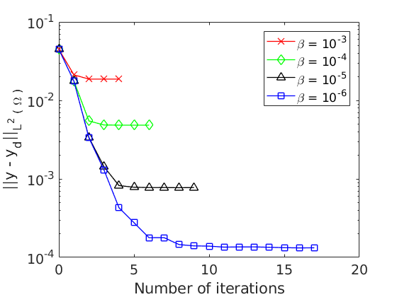
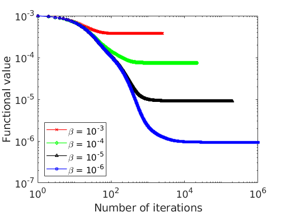
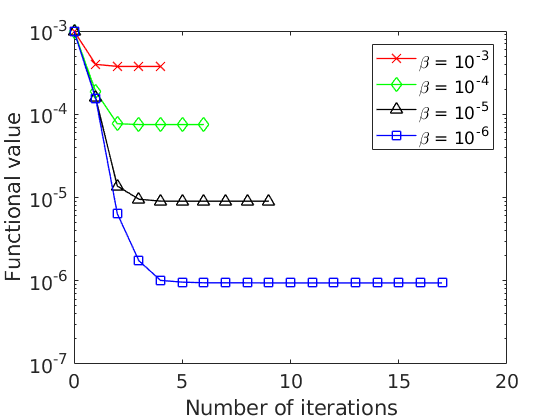
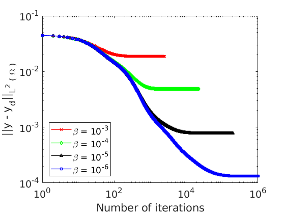
Both solvers, laplaceAdjointFoam for the steepest descent method with $\gamma = 10$ and laplaceCGAdjointFoam for the conjugate gradient method, have been tested in a square domain $[0, 1] \times [0, 1]$ with zero Dirichlet boundary conditions and $\beta = 10^{-3},10^{-4},10^{-5},10^{-6}$. The target function is $y_d = xy \sin \left( \pi x \right) \sin \left( \pi y \right)$.

The problem setup is called case in OpenFOAM and it is independent from the solver itself. A typical case in OpenFOAM has three folders: 0, where the problem fields are stored along with their boundary conditions; constant, that includes the mesh data and the physical properties; and system, with parameters regarding the numerical solution and problem output such as tolerances, linear solvers or write interval. In this example, the case folder is called laplaceAdjointFoamCase.