Introduction
We are interested in optimal control problems subject to a class of diffusion-reaction systems that describes the growth and spread of an introduced population of organisms
\begin{equation} \label{pde}
y_t – y_{xx} = f(y), \quad x\in \mathbb{R}, \quad t \in \mathbb{R}^+,
\end{equation}
where
\begin{equation} \label{fyatet}
f(y)=a y(1-y)(\theta-y),
\end{equation}
is the reaction term that represents local reactions, and $y(t, x) : \mathbb{R}^+ \times \mathbb{R} \rightarrow \mathbb{R}$ is the state of the system. Here $a<0$ and $\theta \in [0,1]$ are two real parameters.
State $y$ represents the local population density. The ``growth'' of $y$ is subject to an Allee effect (described by the reaction term $f$) in addition to migration (described by the term $y_{xx}$). Allee effect exists for a wide variety of reasons such as less efficient feeding at low densities and reduced effectiveness of vigilance and anti-predator defenses.
The value of $|a|$ represents the reproductive rate, and the parameter $\theta \in (0,1)$ is the local critical density or Allee threshold $\theta$ that determines the sign (positive or negative) the population growth. Note that, in some literature, the parameter $\theta$ (Allee threshold) has been supposed to be a dynamic parameter that changes with respect to the evolution of the species. Therefore, by means of biological control (e.g. importation of predators), environmental control (e.g. food supply), modern technology (e.g. DNA manipulations), the birth rate and the Allee threshold should be able to be modified. That is to say, we can consider the parameters $a$ and $\theta$ as the control of the system (\ref{pde}).
Note that the reaction term $f$ has three zeros $0$, $\theta$, and $1$, which correspond to three constant solutions of the system (\ref{pde}).
For system (\ref{pde}), there is a propagation phenomenon: one of the state $y=0$, or $y=1$, or $y=\theta$, propagates in the space.
This phenomenon is generally described by traveling wave solution of the form, \begin{equation} \label{tw}
y(t,x) = Y(x – ct), \quad x \in \mathbb{R}
\end{equation}
which connects two of the three constant solutions of the system (\ref{pde}). Here the constant $c \in \mathbb{R}$ is the wave speed, and $Y$ is called the wave profile. Typically, the wave speed and the wave profile depend on the parameters $a$ and $\theta$.
Given a bounded domain $\Omega \subset \mathbb{R}$, our optimal problem is then to choose optimal (control) parameters $a$ and $\theta$ such that the system (\ref{pde}) goes from a given initial state $y(0,x) = y_0(x) \in [0,1]$, $x\in \Omega$ to a final state $y(T,x)$, $x\in \Omega$ which minimizes the distance between this final state and an expected traveling wave solution $y^d$ of the form (\ref{tw}).
Optimal control problem
We consider the following optimal control problem $(\mathcal{P})_{opt}$.
Let $\Omega=[-L,L]\subset\mathbb{{R}}$ and $T\in\mathbb{{R}^{+}}$ be the given domain and final time, respectively. Find $u=(a,\theta)$ that minimizes the cost functional
\begin{equation}
\label{costfun}
J(u)=\int_{\Omega}|y(T,x)-y^{d}(x)|^{2}dx+K\int_{0}^{T}|\dot{{a}}(t)|^{2}+|\dot{{\theta}}(t)|^{2}dt,
\end{equation}
such that the state $y$ satisfies
\begin{equation}
\label{eqn_difreac}
y_{t}(t,x)-\triangle y(t,x)=f(x,u(t)),\quad (t,x)\in[0,T]\times\Omega,
\end{equation}
$\partial_{x}y(t,x)=0,\quad t\in[0,T],\quad x\in\partial\Omega$ , where $f(x,u(t))=a(t)y(t,x)(1-y(t,x))(\theta(t)-y(t,x))$, and the control $u=(a,\theta)$ satisfies $a(t)\in[a_{min},a_{max}],\quad,\theta(t)\in[\theta_{min},\theta_{max}]\quad t\in[0,T]$, where $y^{d}$ is a desired traveling wave solution of the form (\ref{tw}),
$a_{min},a_{max}$ are non positive constants, and $\theta_{max},\theta_{min}$ are constants between $0$ and $1$.
To solve this problem numerically with AMPL+(an optimization) solver, we need to discretize the problem and transform it into a nonlinear optimization problem.
Let $N_{t}$ and $N_{x}$ be two positive integers. Define a subdivision of time $0=t_{0} Let $K=0.01$, $\delta=0.001$, and the initial data to be a step function, $y_{0}(x)=\begin{cases} In this section, we introduce how to solve the optimal control problem $(\mathcal{P})_{D}$ with AMPL. First, we need to define parameters that will be used, for example, the values of $L,T,N_{t},N_{x}$, etc. After defining all parameters, we can now define the optimal control problem $(\mathcal{P})_{D}$., including the cost functional and all constraints on the state and on the control. Now the optimal control problem is defined, we can finally solve it. Here we use IPOPT solver, which implements a primal-dual To see the optimization result, one can print results into txt files, for example:
\theta_{0}-\delta & x>0\\
0 & x<0
\end{cases}$
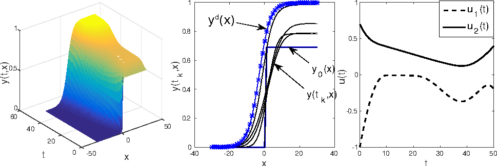
Let us set, moreover, $a\in[-5,0]$. The optimal solution can then be obtained within $10\,s$, and the final cost $J(u)$ is about $5\times10^{-4}$, with its first term $J_{0}(u):=\int_{\Omega}|y(T,x)-y^{d}(x)|^{2}dx=1\times10^{-4}$. The obtained optimal solution is illustrated in the Figure 1. In the right subfigure, $u_{1}=a$ and $u_{2}=\theta$.
[caption id="figure1" align="aligncenter" width="969"] Figure 1: state $y(t,x)$ (left), state $y(\cdot,x)$ (middle), and control $u(t)=(u_1,u_2)$, $u_1=a$, $u_2=\theta$ (right).[/caption]
AMPL code
# Parameters of discretization
param Nt := 250*2;
param Nx := 50;
param L := 30;
param tf := 50;
param dx := 2*L/Nx;
param dt := tf/Nt;
param ymax := 0.6;
set kx ordered := 0..Nx;
set kt ordered := 0..Nt;
param x{j in kx};
let {j in kx} x[j] := -L+j*dx;
param t{i in kt\};
let {i in kt} t[i] := i*dt;

# Parameters of control problem
param u1max := 5; # a_max
param u1min := -5; # a_min
param u2max := 1; # tet_max
param u2min := 0; # tet_min
param tet0 := 0.7;
param tetf := 0.4;
param a0 := -1;
param af := -0.2;
param Ktet := 0.01;
param Ka := 0.01;
param x1 := 0;

# Parameters of initial data
param A0 := sqrt(-a0);
param c0 := -A0*sqrt(2)*(1/2-tet0);
param y0 {j in kx};
let {j in 0..Nx/2} y0[j] := 0;
let {j in Nx/2+1..Nx} y0[j] := tet0-0.01;

# Parameters of desired solution
param Af := sqrt(-af);
param cf := -Af*sqrt(2)*(1/2-tetf);
param yobj{i in kx};
param x2 := x1+cf*Nt*dt;
let {j in kx} yobj[j] := 0.35 ;

# Parametre for initialisation \par
# (0 => rien; 1 => constant; 2 => init.txt)
param Init_Type = 1;
# Declare the variables and their bounds
var a{i in kt} >= u1min, <= u1max;
var tet{i in kt} >= u2min, <= u2max;
var y{i in kt, j in kx} >= 0, <= 1;

# Specify the objective function
minimize obj: sum{j in kx} ( ( y[Nt,j] - yobj[j])$\textasciicircum{}2$
+ Ktet*sum{j in kt diff{0}} (tet[j]-tet[j-1])$\textasciicircum{}2$
+ Ka*sum{j in kt diff{0}} (a[j]-a[j-1])$\textasciicircum{}2;$
# Contraints of the control
subject to c1: tet[0] - tet0 = 0;
subject to c2: a[0] - a0 = 0;
subject to c3: tet[Nt] - tetf = 0;
subject to c4: a[Nt] - af = 0;

# Initial data
subject to i1 {j in kx}: y[0,j] = y0[j] ;

# Dynamical constraints (Backward )
subject to d1 {i in kt diff{Nt}, j in kx diff {0,Nx}}:
  (y[i+1,j] - y[i,j]) - 1/2*dt*( y[i+1,j+1]-2*y[i+1,j]+
  y[i+1,j-1]+y[i,j+1]-2*y[i,j]+y[i,j-1])/$dx\textasciicircum{}2$-
  1/2*dt*( a[i+1]*y[i+1,j]*(1 - y[i+1,j]) *(tet[i+1]- y[i+1,j])+
  a[i]*y[i,j]*(1 - y[i,j]) *(tet[i]- y[i,j])) = 0;

# Boundary constraints
subject to b1 {i in kt diff{0}}: y[i,1] - y[i,0] = 0;
subject to b2 {i in kt diff{0}}: y[i,Nx] - y[i,Nx-1] = 0;
# Initialization of state and control variables
if (Init_Type == 1) then {
  let {j in kt} tet[j] := tetf;
  let {j in kt} a[j] := 0;
  for {i in kt diff{0},j in kx}{
   let y[i,j] := ymax*exp(Af*(-L+j*dx-cf*i*dt)/sqrt(2))/
     (1 + exp(Af*(-L+j*dx-cf*i*dt)/sqrt(2)));
  }
};
# Initialisation avec $\textquotedbl{}init.txt\textquotedbl{} $(only state and control)
if (Init_Type == 2) then {
  read {i in kt} (a[i],tet[i]) < init.txt;
 read {i in kt, j in kx} (y[i,j]) < init.txt;
};
interior point method. Recall that an interior point method is a linear or nonlinear programming method. Of course, one can also choose other appropriate optimization solvers.
# tell ampl to use the ipopt executable as a solver
# make sure ipopt is in the path!
option solver ipopt;

# solve the problem option
ipopt_options 'max_iter=1000
tol=1e-6';
solve;
# print the solution to out.txt
option display_precision 6;
printf: $\textquotedbl{}obj=\textquotedbl{} >>\textcompwordmark{}$ out.txt;
printf: $\textquotedbl{} \%24.16e; \textbackslash{}n\textquotedbl{},
obj >>\textcompwordmark{}$ out.txt;
Authors: Jiamin ZHU & Enrique Zuazua
December, 2017

