
PDF version | Download Matlab Code…
Introduction
We introduce the following notation: $L^2=L^2\left(\Omega\right)$, $L^2_T=L^2\left(\Omega\times \left(0,T\right)\right)$,
\begin{eqnarray*}
\langle u,v \rangle&=&\int_{\Omega}^{} u(x)v(x) \ dx;\\
\langle u,v \rangle_T^2&=&\int_{0}^{T} \int_{\Omega}^{} u(x,t)v(x,t) \ dx \ dt
\end{eqnarray*}
and the correspondent norms $\norm{\cdot}=\langle \cdot,\cdot\rangle$ and $\norm{\cdot}_T=\langle \cdot,\cdot\rangle_T$. Moreover, we define the norms
\begin{eqnarray*}
\norm{v}_{1}&=&\int_{\Omega}^{} \abs{v(x)} \ dx;\\
\norm{v}_{1,T}&=&\int_{0}^{T} \int_{\Omega}^{} \abs{v(x,t)} \ dx \ dt.
\end{eqnarray*}
We want to study the following optimal control problem:
\begin{equation*}
\left(\mathcal{P}\right) \ \ \ \ \ \ \ \hat{u}\in\argmin_{u\in L^2_T} \left\{J\left(u\right)=\alpha_c \norm{u}_{1,T} + \frac{\beta}{2}\norm{u}^2_{T}+\alpha_s \norm{Lu}_{1,T} + \frac{\gamma}{2}\norm{Lu-z}_{T}^2\right\},
\end{equation*}
where $L: \ L^2_T \to L^2_T$ is defined by
\begin{eqnarray*}
Lu&=&y
\end{eqnarray*}
and $y$ is the solution of the PDE given by
\begin{equation*}
\begin{cases}
y’+Ay=Bu & \left(\Omega \times \left(0,T\right)\right)\\
y=0 & \left(\partial\Omega\times \left(0,T\right)\right)\\
y(0)=0 & \left(\Omega\right).
\end{cases}
\end{equation*}
Notice that, by integration by parts, $L^*\mu=B^* p$, where $\varphi$ is solution of the adjoint equation:
\begin{equation*}
\begin{cases}
-p’+A^* p =\mu & \left(\Omega \times \left(0,T\right)\right)\\
p=0 & \left(\partial\Omega\times \left(0,T\right)\right)\\
p(T)=0 & \left(\Omega\right).
\end{cases}
\end{equation*}
Sparse control: $\alpha_c>0$ ($\alpha_s=0$)
The stationary problem
\begin{equation*}
\left(\mathcal{S}\mathcal{P}_c\right) \ \ \ \ \ \ \ \bar{u}\in\argmin_{u\in L^2} \left\{J_s\left(u\right)=\alpha_c \norm{u}_{1} + \frac{\beta}{2}\norm{u}^2+ \frac{\gamma}{2}\norm{y-z}^2: \ \ \ Ay=Bu \right\}.
\end{equation*}
Optimality conditions
\begin{equation*}
\begin{cases}
A\bar{y}=B \ shrink(-B^*\bar{p},\frac{\alpha_c}{\beta}) & \left(\Omega\right)\\
A^*\bar{p}=\gamma\left(\bar{y}-z\right) & \left(\Omega\right)\\
\bar{y}=0, \ \bar{p}=0 & \left(\partial\Omega\right).
\end{cases}
\end{equation*}
Numerical algorithm
In order to compute a numerical solution of problem $\left(\mathcal{S}\mathcal{P}_c\right)$, after a discretization by finite differences, we use a prox-prox splitting: first write the state as $y=A^{-1}Bu$, then
- Proximal-point step:
- Proximal-point step:
\begin{equation*}
\begin{split}
\tilde{u}_{k} & =\argmin_{u\in L^2} \left\{\frac{\beta}{2}\norm{u}^2 + \frac{\gamma}{2}\norm{A^{-1}Bu-z}^2+ \frac{1}{2\lambda_k}\norm{u-u_k}^2\right\}\\
& = \left[\left(\beta+\frac{1}{\lambda_k}\right)I+\gamma B^*A^{-*}A^{-1}B\right]^{-1}\left(\frac{1}{\lambda_k}u_k+\gamma B^*A^{-*}z\right).
\end{split}
\end{equation*}
\begin{equation*}
\begin{split}
u_{k+1}& =\argmin_{u\in L^2} \left\{\alpha_c \norm{u}_{1,T} + \frac{1}{2\lambda_k}\norm{u-\tilde{u}_k}_{T}^2\right\}\\
& = shrink(\tilde{u}_k,\alpha_c \lambda_k).
\end{split}
\end{equation*}
Remark: Notice that, when $\alpha_s=0$, the solution of $\left(\mathcal{P}^c_s\right)$ is simply given by
$$\bar{u}=\gamma \left[\beta I+\gamma B^*A^{-*}A^{-1}B\right]^{-1}B^*A^{-*}z.$$
Evolutionary problem
\begin{equation*}
\left(\mathcal{P}_c\right) \ \ \ \ \ \ \ \hat{u}\in\argmin_{u\in L^2_T} \left\{J\left(u\right)=\alpha_c \norm{u}_{1,T} + \frac{\beta}{2}\norm{u}^2_{T} + \frac{\gamma}{2}\norm{Lu-z}_{T}^2\right\}.
\end{equation*}
Optimality conditions
Define the classical Lagrangian
\begin{equation*}
\begin{split}
\mathcal{L}\left(u,y,p\right)&=J\left(u\right)+\langle p, Bu-y’-Ay\rangle_T.
\end{split}
\end{equation*}
By integration by parts, we have
\begin{equation*}
\begin{split}
\mathcal{L}\left(u,y,p\right)&=\alpha_c \norm{u}_{1,T} + \frac{\beta}{2}\norm{u}^2_{T}+ \frac{\gamma}{2}\norm{y-z}_{T}^2 + \langle B^*p, u\rangle_T \\
& \quad + \langle p’-A^*p,y\rangle_T + \langle p(0),y(0)\rangle – \langle p(T),y(T)\rangle.
\end{split}
\end{equation*}
Deriving with respect to the three variables $\left(u,y,p\right)$, we obtain the optimality system:
\begin{equation*}
\begin{cases}
\hat{y}’+A\hat{y}=B\hat{u} & \left(\Omega \times \left(0,T\right)\right)\\
-\hat{p}’+A^*\hat{p}=\gamma\left(y-z\right) & \left(\Omega \times \left(0,T\right)\right)\\
\hat{y}=0, \ \hat{p}=0 & \left(\partial\Omega\times \left(0,T\right)\right)\\
\hat{y}(0)=0, \ \hat{p}(T)=0 & \left(\Omega\right),
\end{cases}
\end{equation*}
where the relation between the optimal control and the dual state is given by
\begin{equation*}
0\in \alpha_c \ \partial \norm{\cdot}_{1,T} \left(\hat{u}\right) + \beta \hat{u} + B^*\hat{p}.
\end{equation*}
The latter is equivalent to
\begin{equation*}
\begin{split}
\hat{u}&=\left(\beta I+\alpha_c \ \partial \norm{\cdot}_{1,T} \right)^{-1}\left(-B^*\hat{p}\right)\\
&=\argmin_{v\in L^2_T} \left\{ \alpha_c \norm{v}_{1,T}+\frac{1}{2\beta}\norm{v+B^*\hat{p}}_T^2 \right\}\\
&=shrink(-B^*\hat{p},\frac{\alpha_c}{\beta}),
\end{split}
\end{equation*}
where the operator of $soft-shrinkage$ is defined by
\begin{equation*}
shrink(t,\alpha)=
\begin{cases}
t+\alpha & (t<-\alpha)\\
0 & (-\alpha\leq t \leq \alpha)\\
t-\alpha & (t>\alpha).
\end{cases}
\end{equation*}
Finally,
\begin{equation*}
\begin{cases}
\hat{y}’+A\hat{y}=B \ shrink(-B^*\hat{p},\frac{\alpha_c}{\beta})& \left(\Omega \times \left(0,T\right)\right)\\
-\hat{p}’+A^*\hat{p}=\gamma\left(y-z\right) & \left(\Omega \times \left(0,T\right)\right)\\
\hat{y}=0, \ \hat{p}=0 & \left(\partial\Omega\times \left(0,T\right)\right)\\
\hat{y}(0)=0, \ \hat{p}(T)=0 & \left(\Omega\right).
\end{cases}
\end{equation*}
Numerical algorithm
In order to compute a numerical solution of problem $\left(\mathcal{P}_c\right)$, after a discretization by finite differences, we use a grad-prox splitting:
- Gradient step:
- Proximal-point step:
\begin{equation*}
\begin{split}
\tilde{u}_{k} & = u_k-\lambda_k \nabla_u \left[\frac{\beta}{2}\norm{u}^2_{T} + \frac{\gamma}{2}\norm{Lu-z}_{T}^2 \right]\left(u_k\right) \\
& = u_k-\lambda_k \left[\beta u_k+\gamma L^*\left(Lu_k-z\right)\right]\\
& = u_k – \lambda_k\left[\beta u_k+\gamma B^*p_k\right],
\end{split}
\end{equation*}
where
\begin{equation*}
\begin{cases}
y_k’+Ay_k=Bu_k & \left(\Omega \times \left(0,T\right)\right)\\
y_k=0 & \left(\partial\Omega\times \left(0,T\right)\right)\\
y_k(0)=0 & \left(\Omega\right)
\end{cases}
\end{equation*}
and
\begin{equation*}
\begin{cases}
-p_k’+A^* p_k =y_k-z & \left(\Omega \times \left(0,T\right)\right)\\
p_k=0 & \left(\partial\Omega\times \left(0,T\right)\right)\\
p_k(T)=0 & \left(\Omega\right).
\end{cases}
\end{equation*}
\begin{equation*}
\begin{split}
u_{k+1}& =\argmin_{u\in L^2_T} \left\{\alpha_c \norm{u}_{1,T} + \frac{1}{2\lambda_k}\norm{u-\tilde{u}_k}_{T}^2\right\}\\
& = shrink(\tilde{u}_k,\alpha_c \lambda_k).
\end{split}
\end{equation*}
Remarks: Another possibility is to include the term $\frac{\beta}{2}\norm{u}^2_{T}$ in the proximal step.
Notice that, for $$f(u)=\frac{\beta}{2}\norm{u}^2_{T} + \frac{\gamma}{2}\norm{Lu-z}_{T}^2,$$
then $\nabla f$ is Lipschitz continuous. Indeed, for $u_i\in L^2_T$ ($i=1,2$), then
$$\nabla f (u_i)=\beta u_i+\gamma B^{*}p_i,$$
where
\begin{equation*}
\begin{cases}
y_i’+Ay_i=Bu_i & \left(\Omega \times \left(0,T\right)\right)\\
y_i=0 & \left(\partial\Omega\times \left(0,T\right)\right)\\
y_i(0)=0 & \left(\Omega\right)
\end{cases}
\end{equation*}
and
\begin{equation*}
\begin{cases}
-p_i’+A^* p_i=y_i-z & \left(\Omega \times \left(0,T\right)\right)\\
p_i=0 & \left(\partial\Omega\times \left(0,T\right)\right)\\
p_i(T)=0 & \left(\Omega\right).
\end{cases}
\end{equation*}
By linearity $\delta y=y_2-y_1$ and $\delta p=p_2-p_1$ solve the same equations with right-hand-sides $B(u_2-u_1)$ and $\delta y$, respectively. Then
\begin{equation*}
\begin{split}
\norm{\nabla f(u_2)-\nabla f(u_1)}&\leq \beta\norm{u_2-u_1}_T + \gamma \norm{B^*}\norm{\delta p}_T\\
&\leq \beta\norm{u_2-u_1}_T + \gamma \ C_{adj} \norm{B} \norm{\delta y}_T\\
& \leq \beta\norm{u_2-u_1}_T + \gamma \ C_{adj} C \ \norm{B} \norm{B(u_2-u_1)}_T\\
& \leq L \norm{u_2-u_1}_T,
\end{split}
\end{equation*}
where we defined
$$L=\beta+\gamma \ C_{adj} C \ \norm{B}^2.$$
In order the prox-grad method to converge, the restriction on the step size is given by
$$0<\lambda \leq \lambda_k \leq \Lambda <\frac{2}{L}.$$
Sparse state: $\alpha_s>0$ ($\alpha_c=0$)
\begin{equation*}
\left(\mathcal{P}_s\right) \ \ \ \ \ \ \ \hat{u}\in\argmin_{u\in L^2_T} \left\{J\left(u\right)=\frac{\beta}{2}\norm{u}^2_{T}+\alpha_s \norm{Lu}_{1,T} + \frac{\gamma}{2}\norm{Lu-z}_{T}^2\right\}.
\end{equation*}
The stationary problem
\begin{equation*}
\left(\mathcal{S}\mathcal{P}_s\right) \ \ \ \ \ \ \ \bar{u}\in\argmin_{u\in L^2} \left\{J_s\left(u\right)=\alpha_c \norm{u}_{1} + \frac{\beta}{2}\norm{u}^2+ \frac{\gamma}{2}\norm{y-z}^2: \ \ \ Ay=Bu \right\}.
\end{equation*}
Optimality conditions
\begin{equation*}
\begin{cases}
A\bar{y}=-\frac{1}{\beta}BB^*\hat{p} & \left(\Omega \times \left(0,T\right)\right)\\
\hat{y}=shrink(A^*\hat{p}+\gamma z,\frac{\alpha_s}{\gamma}) & \left(\Omega \times \left(0,T\right)\right)\\
\bar{y}=0, \ \bar{p}=0 & \left(\partial\Omega\times \left(0,T\right)\right).
\end{cases}
\end{equation*}
Finally, we obtain a single equation in the dual variable $p$:
\begin{equation*}
\begin{cases}
A \ shrink(A^*\bar{p}+\gamma z,\frac{\alpha_s}{\gamma})=-\frac{1}{\beta}BB^*\bar{p} & \left(\Omega \times \left(0,T\right)\right)\\
\bar{p}=0 & \left(\partial\Omega\times \left(0,T\right)\right).
\end{cases}
\end{equation*}
Numerical algorithm
In order to compute a numerical solution of problem $\left(\mathcal{P}_s\right)$, after a discretization by finite differences, we use a prox-prox splitting on the Augmented Energy: first write the state as $y=A^{-1}Bu$, then
- Proximal-point step:
- Proximal-point step:
\begin{equation*}
\begin{split}
u_{k+1} & =\argmin_{u\in L^2} \left\{\frac{\beta}{2}\norm{u}^2 + \frac{\gamma}{2}\norm{A^{-1}Bu-z}^2+\frac{\delta}{2\lambda_k}\norm{A^{-1}Bu-y_k}^2 +\frac{1}{2\lambda_k}\norm{u-u_k}^2\right\}\\
& = \left[\left(\beta+\frac{1}{\lambda_k}\right)I+\left(\gamma+\frac{\delta}{\lambda_k}\right) B^*A^{-*}A^{-1}B\right]^{-1}\left[\frac{1}{\lambda_k}u_k+ B^*A^{-*}\left(\gamma z+\frac{\delta}{\lambda_k}y_k\right)\right].
\end{split}
\end{equation*}
\begin{equation*}
\begin{split}
y_{k+1}& =\argmin_{y\in L^2} \left\{
\alpha_s \norm{y}_{1} + \frac{\delta}{2\lambda_k}\norm{y-A^{-1}Bu_{k+1}}^2+\frac{1}{2\lambda_k}\norm{y-y_k}_{T}^2\right\}\\
& = shrink(\tilde{y}_k,\tilde{\lambda}_k),
\end{split}
\end{equation*}
where we defined
\begin{eqnarray*}
\tilde{y}_k & = & \frac{y_k+\delta A^{-1}B u_{k+1}}{1+\delta};\\
\tilde{\lambda}_k & = & \frac{\alpha_s \lambda_k}{1+\delta}.
\end{eqnarray*}
Remark: Notice that again, when $\alpha_s=0$, the solution of $\left(\mathcal{P}_s\right)$ is simply given by
$$\bar{u}=\gamma \left[\beta I+\gamma B^*A^{-*}A^{-1}B\right]^{-1}B^*A^{-*}z.$$
Evolutionary problem
Optimality conditions
Define the classical Lagrangian
\begin{equation*}
\begin{split}
\mathcal{L}\left(u,y,p\right)&=J\left(u\right)+\langle p, Bu-y’-Ay\rangle_T.
\end{split}
\end{equation*}
By integration by parts, we have
\begin{equation*}
\begin{split}
\mathcal{L}\left(u,y,p\right)&=\frac{\beta}{2}\norm{u}^2_{T}+\alpha_s \norm{y}_{1,T} + \frac{\gamma}{2}\norm{y-z}_{T}^2 + \langle B^*p, u\rangle_T \\
& \quad + \langle p’-A^*p,y\rangle_T + \langle p(0),y(0)\rangle – \langle p(T),y(T)\rangle.
\end{split}
\end{equation*}
Deriving with respect to the three variables $\left(u,y,p\right)$, we obtain the optimality system:
\begin{equation*}
\begin{cases}
\hat{y}’+A\hat{y}=B\hat{u} & \left(\Omega \times \left(0,T\right)\right)\\
-\hat{p}’+A^*\hat{p}\in\gamma\left(\hat{y}-z\right)+\alpha_s \ \partial \norm{\cdot}_{1,T} \left(\hat{y}\right) & \left(\Omega \times \left(0,T\right)\right)\\
\hat{y}=0, \ \hat{p}=0 & \left(\partial\Omega\times \left(0,T\right)\right)\\
\hat{y}(0)=0, \ \hat{p}(T)=0 & \left(\Omega\right),
\end{cases}
\end{equation*}
where the relation between the optimal control and the dual state is given by
\begin{equation*}
\hat{u} = -\frac{1}{\beta}B^*\hat{p}.
\end{equation*}
The adjoint equation is equivalent to
\begin{equation*}
\begin{split}
\hat{y}&=\left(\gamma I+\alpha_s \ \partial \norm{\cdot}_{1,T} \right)^{-1}\left(-\hat{p}’+A^*\hat{p}+\gamma z\right)\\
&=shrink(-\hat{p}’+A^*\hat{p}+\gamma z,\frac{\alpha_s}{\gamma}).
\end{split}
\end{equation*}
Finally,
\begin{equation*}
\begin{cases}
\hat{y}’+A\hat{y}=-\frac{1}{\beta}B B^*\hat{p} & \left(\Omega \times \left(0,T\right)\right)\\
\hat{y}=shrink(-\hat{p}’+A^*\hat{p}+\gamma z,\frac{\alpha_s}{\gamma}) & \left(\Omega \times \left(0,T\right)\right)\\
\hat{y}=0, \ \hat{p}=0 & \left(\partial\Omega\times \left(0,T\right)\right)\\
\hat{y}(0)=0, \ \hat{p}(T)=0 & \left(\Omega\right),
\end{cases}
\end{equation*}
Numerical algorithm
In order to compute a numerical solution of problem $\left(\mathcal{P}_s\right)$, after a discretization by finite differences, we use a grad-prox splitting on the following Augmented Energy:
\begin{equation*}
\mathcal{L}_{\lambda}\left(u,y\right)=\frac{\beta}{2}\norm{u}^2_{T}+\alpha_s \norm{y}_{1,T}+ \frac{\gamma}{2}\norm{Lu-z}_{T}^2+\frac{\delta}{2\lambda}\norm{Lu-y}_{T}^2.
\end{equation*}
Then,
- Gradient step:
- Proximal-point step:
- Spacial domain: $\Omega=\left(0,1\right)$;
- Time interval: $\left[0,T\right]$, with $T=1$;
- Weight-parameters: $\alpha_c=[0, 0.01]$, $\alpha_s=[0, 0.65]$, $\beta=0.0001$ and $\gamma=1$;
- Trajectory target: $$z(x)=\mathcal{I}_{\left[x_a,x_b\right]},$$ where $x_a=1.7/3$, $x_b=3.5/4$;
- Control operator: for $x_1=1/7$ and $x_2=4/5$,
$$B=\mathcal{I}_{\left[x_1,x_2\right]};$$ - $A$ is the finite difference discretization of $-\Delta$;
- Numerical grid: $N_x=300$ in space, $N_t=100$ in time.
\begin{equation*}
\begin{split}
u_{k+1} & = u_k-\lambda_k \nabla_u \left[\frac{\beta}{2}\norm{u}^2_{T}+ \frac{\gamma}{2}\norm{Lu-z}_{T}^2+\frac{\delta}{2\lambda}\norm{Lu-y}_{T}^2 \right]\left(u_k\right) \\
& = u_k-\lambda_k \left[\beta u_k+\gamma L^*\left(Lu_k-z\right)+\frac{\delta}{\lambda_k}L^*\left(Lu_k-y_k\right)\right]\\
& = \left(1-\beta\lambda_k\right)u_k – B^*p_k,
\end{split}
\end{equation*}
where
\begin{equation*}
\begin{cases}
y_{u_k}’+Ay_{u_k}=Bu_k & \left(\Omega \times \left(0,T\right)\right)\\
y_{u_k}=0 & \left(\partial\Omega\times \left(0,T\right)\right)\\
y_{u_k}(0)=0 & \left(\Omega\right)
\end{cases}
\end{equation*}
and
\begin{equation*}
\begin{cases}
-p_k’+A^* p_k =\left(\gamma \lambda_k + \delta\right)y_{u_k}-\gamma \lambda_k z – \delta y_k & \left(\Omega \times \left(0,T\right)\right)\\
p_k=0 & \left(\partial\Omega\times \left(0,T\right)\right)\\
p_k(T)=0 & \left(\Omega\right).
\end{cases}
\end{equation*}
\begin{equation*}
\begin{split}
y_{k+1}& =\argmin_{y\in L^2_T} \left\{\alpha_s \norm{y}_{1,T} + \frac{\delta}{2\lambda_k}\norm{y-Lu_{k+1}}_T^2+\frac{1}{2\lambda_k}\norm{y-y_k}_{T}^2\right\}\\
& = shrink(\tilde{y}_k,\tilde{\lambda}_k),
\end{split}
\end{equation*}
where we defined
\begin{eqnarray*}
\tilde{y}_k & = & \frac{y_k+\delta L u_{k+1}}{1+\delta};\\
\tilde{\lambda}_k & = & \frac{\alpha_s \lambda_k}{1+\delta}.
\end{eqnarray*}
-
Remark: Another possibility is to consider
\begin{equation*}
\mathcal{L}_{\lambda}\left(u,y\right)=\frac{\beta}{2}\norm{u}^2_{T}+\alpha_s \norm{y}_{1,T}+ \frac{\gamma}{2}\norm{y-z}_{T}^2+\frac{\delta}{2\lambda}\norm{Lu-y}_{T}^2.
\end{equation*}
Computational experiments
In the following, we present the setting for the numerical experiments.
Stationary solutions
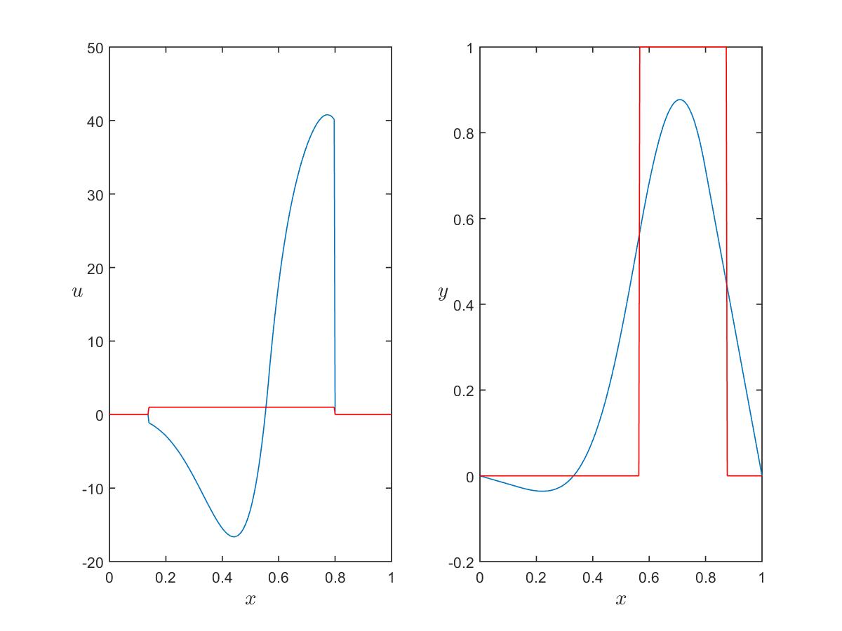
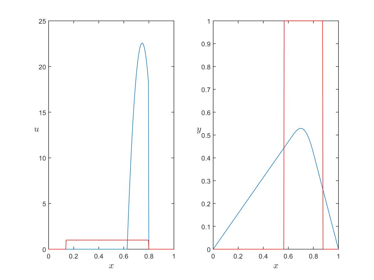
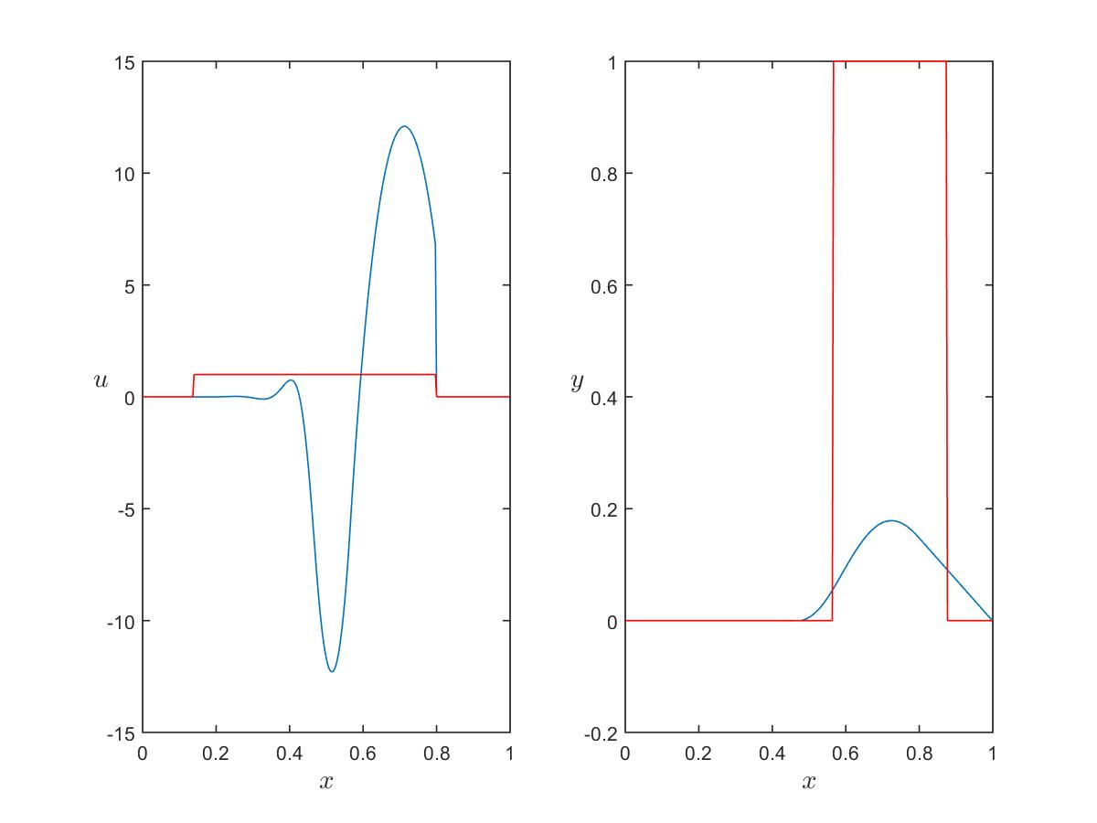
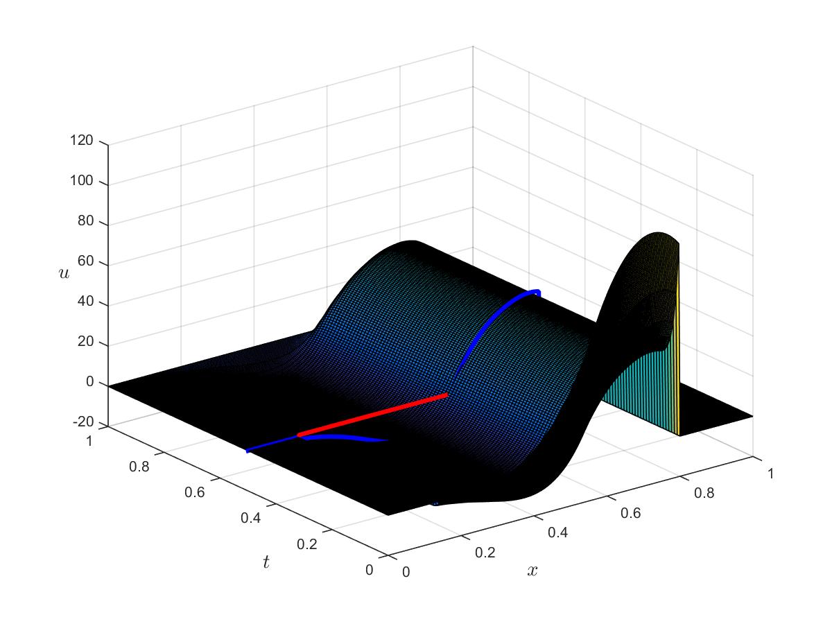
Evolutionary problem
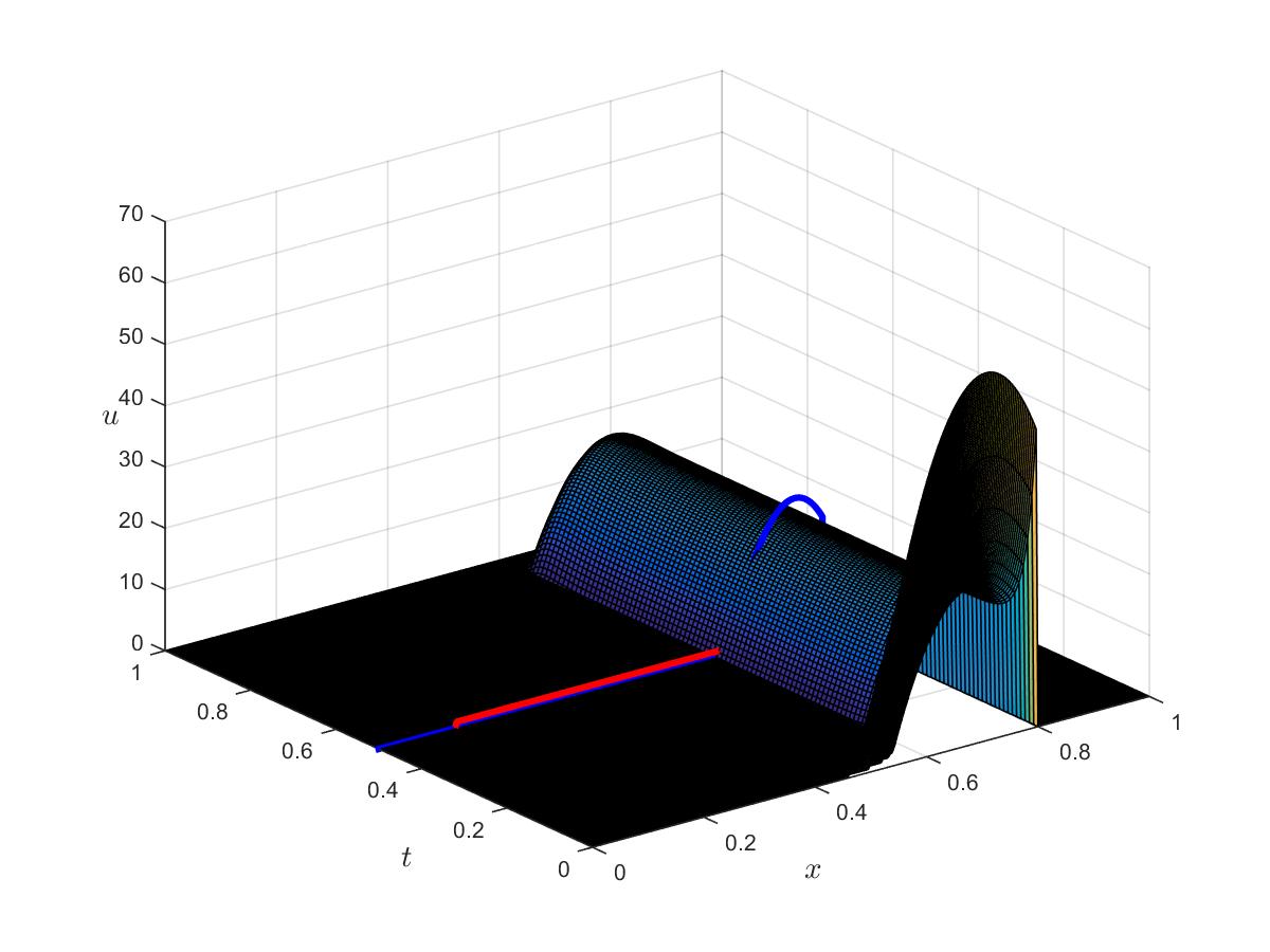
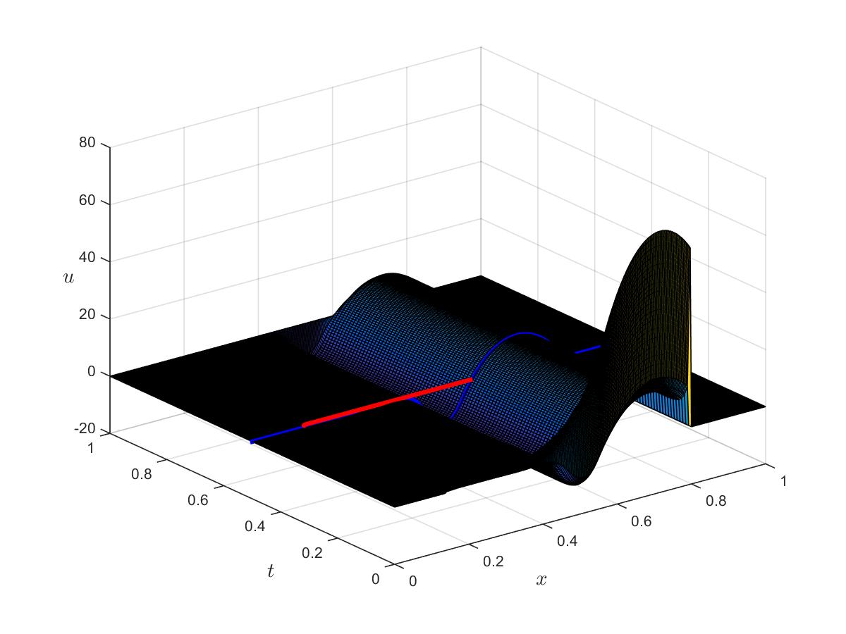
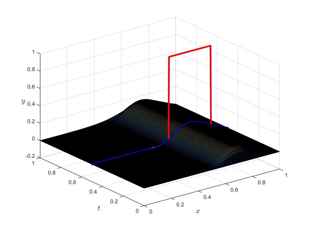
Optimal control
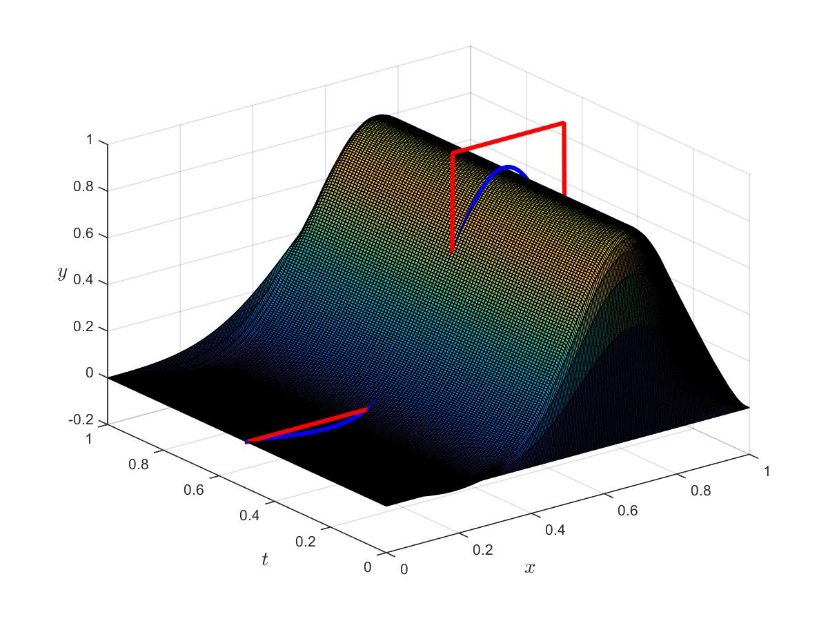
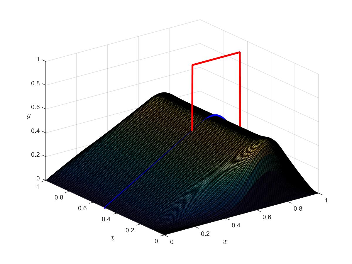
Optimal state
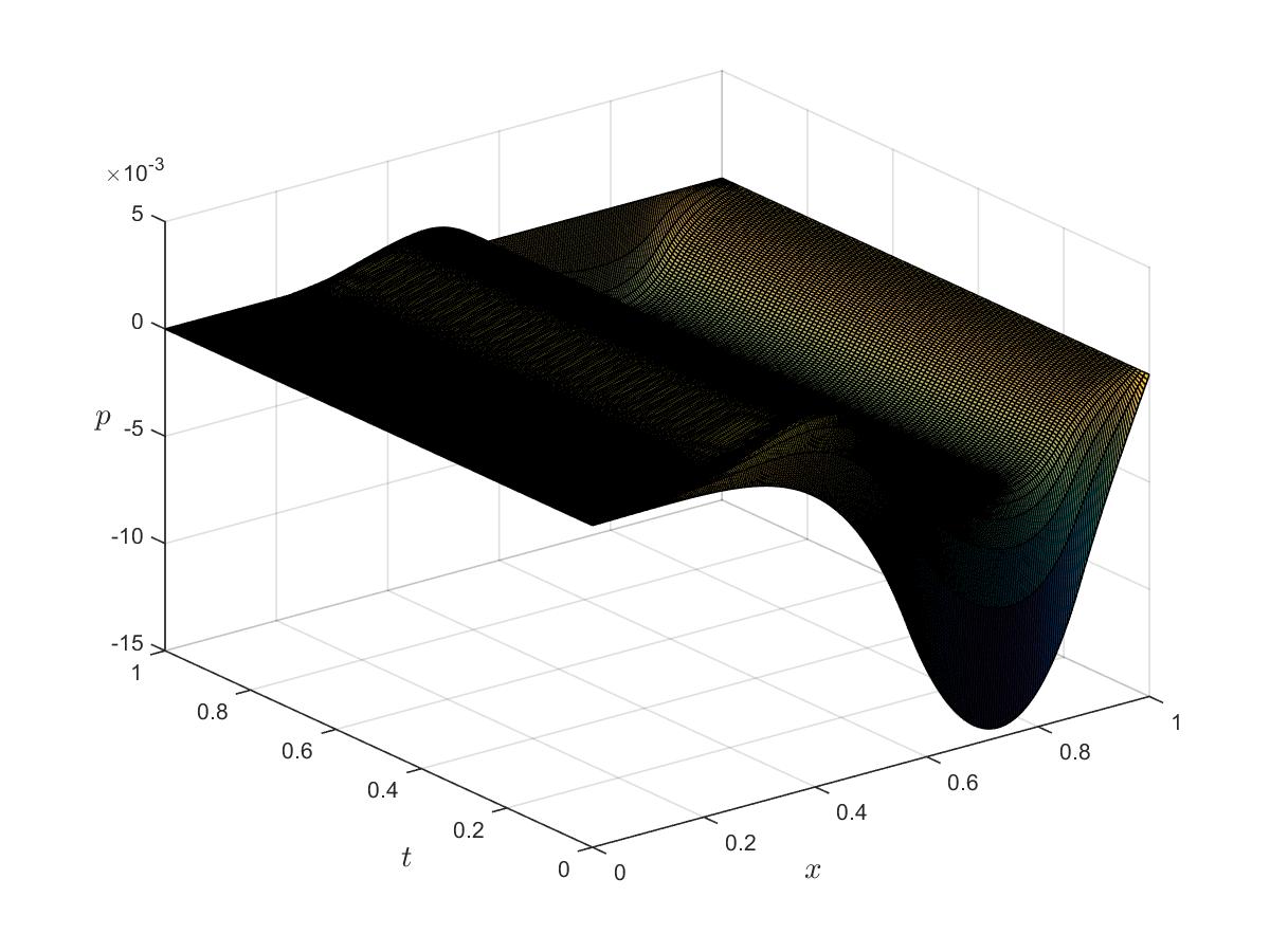
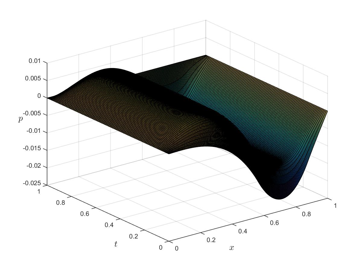
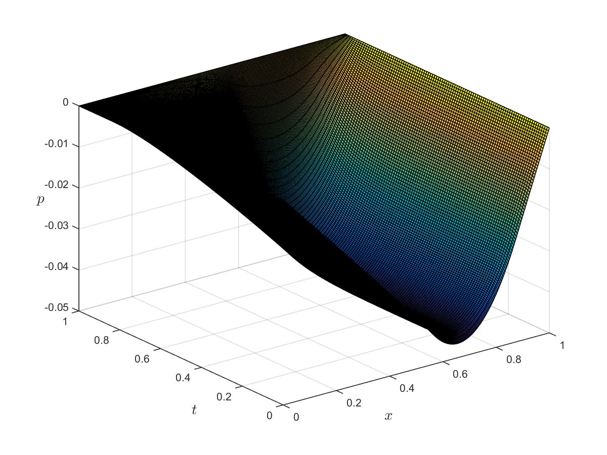
Optimal adjoint
Bibliography
[1] Peypouquet, J. Convex optimization in normed spaces: theory, methods and examples. With a foreword by Hedy Attouch. Springer Briefs in Optimization. Springer, Cham, 2015. xiv+124 pp.

