
Date: September 01, 2026
Good Solutions, Bad Coordinates: The Coercivity Gap in Neural Partial Differential Equation Solvers
Author: Enrique Zuazua
Sometimes, a neural partial differential equation (PDE) solver may appear to be misbehaving, in that some weights grow without apparent bound as neurons collapse onto one another. In many numerical settings, such behavior would seem like a warning sign of instability, poor conditioning, or impending failure. In neural approximation, however, the diagnosis can be subtler: the coordinates may deteriorate while the computed physical field remains accurate.
This distinction matters because while parameter growth is often interpreted as numerical failure, in some neural PDE solvers it may instead signal that the architecture is approaching a legitimate state-space limit that lies outside of its finite parametrization. It matters even more as scientific machine learning (ML) becomes part of the numerical toolbox for PDEs and ordinary differential equations. Physics-informed neural networks (PINNs), deep Ritz methods, operator learning, and related techniques use trainable functions to encode physical laws, data, boundary conditions, and variational principles; representative entry points are the deep Ritz method [1] and the broader physics-informed ML framework [2]. These methods are especially appealing in high-dimensional settings, where classical grids can become prohibitively expensive.
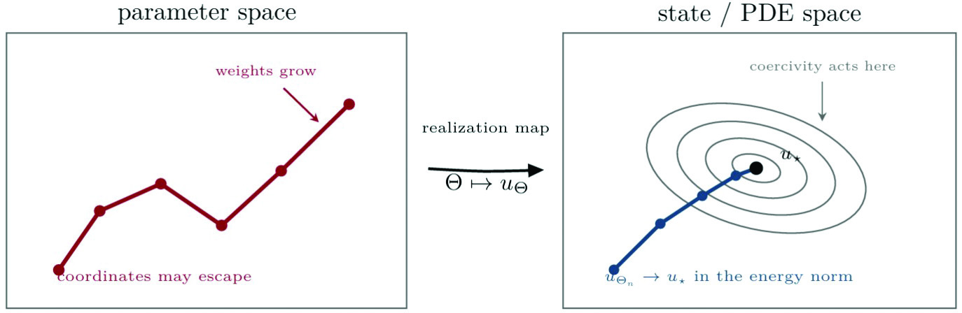
Figure 1. The optimizer moves in parameter space while the partial differential equation energy or residual acts on the realized state. Coercivity controls the state, but not necessarily its coordinates. Figure courtesy of Ziqian Li.
The central question is familiar to numerical analysts but newly delicate in this setting: What exactly must converge? The optimizer evolves weights, biases, centers, and other parameters, but the differential equation only sees the realized physical state. The coercivity gap [4] names the separation between these two worlds; a neural PDE solver can produce states that converge even while the parameters that generate them diverge. Figure 1 summarizes this basic tension where the optimizer moves in parameter space, while the PDE judges the realized state.
Two Traditions Meet
For many years, ML and scientific computing developed along different paths. Neural networks grew out of questions in learning, statistics, and pattern recognition, and eventually large-scale data applications such as vision, speech, and language. Conversely, scientific computing developed around the numerical approximation of differential equations through finite differences, finite elements, spectral methods, and variational techniques.
A large part of the classical route was shaped by variational formulations of PDEs. Approximation properties, stability estimates, compactness, and coercivity became the standard tools that explain why a numerical method should converge. These ideas were typically developed for trial spaces with a transparent linear structure.
The combination of these traditions created scientific ML. Neural networks became nonlinear approximation spaces for PDEs, while optimization algorithms from ML became practical tools for minimizing residuals or energies. Universal approximation results suggested expressive power; physical models supplied structure and data supplied additional constraints. This is part of a larger dialogue between control, learning, and computation [3].
However, the meeting also changed the mathematical objects under observation. In a classical finite element method, the unknown coefficient vector and the approximate solution are tightly linked through a fixed linear basis. In a neural method, the unknowns live in parameter space, while the PDE stability theory lives in function space.
The Coercivity Gap
Consider the usual Galerkin picture; a coercive elliptic energy is minimized over a finite-dimensional linear space. If the basis is fixed, bounded coefficients produce bounded approximate states, and the discrete minimizer exists in the trial space. The coefficient vector and the physical field remain closely tied to each other.
Neural approximation changes this point. The trial object is no longer a linear space; it is the image of a nonlinear realization map:
\Theta \mapsto u_{\Theta}
Here, \Theta denotes the trainable parameters, while u_{\Theta} is the physical state. The PDE does not see \Theta directly, it only recognizes u_{\Theta}.
Both viewpoints are natural. From the ML side, attention is directed toward the trajectory of weights, biases, centers, and learning rates. From the PDE side, the primary object is the field that solves the equation in an energy or stability norm. For classical linear discretization, these views often lead to the same conclusion. However, neural parametrizations can separate them.
This distinction is harmless when the realization map is compact and well behaved. It becomes decisive when the image of the map is not closed. In this case, a sequence of neural states may converge to a perfectly regular function that need not be represented by any finite parameter vector of the chosen architecture.
Coercivity reenters on the state side. It may control the error in the energy norm, or a stability estimate may control the state from a residual. Yet such control need not imply boundedness, compactness, or convergence of \Theta Stability can get lost in parameter space and recovered in state space.
Two Neurons Are Enough
A fixed-width Gaussian example makes the point visible. Let G(x) = \exp(-x^2/4) up to an irrelevant normalization, and place two Gaussian neurons symmetrically around the origin. With opposite weights of size 1/(2h) their realized state is the centered difference quotient
q_h(x) = \frac{G(x+h) - G(x-h)}{2h} \to G'(x) \quad \text{as } h \to 0.
As h approaches zero, the two centers collide, and the two weights become unbounded. Nevertheless, q_h converges to the derivative of a Gaussian in the natural Sobolev norms. The parameters escape but the physical state converges; see Figure 2 for an illustration of this collision mechanism.
This is not merely a redundancy of the parametrization. The two neurons are active for every h>0. In this fixed-width Gaussian model—as proved in a detailed mathematical analysis of this mechanism [4]—the limiting state lies in the closure of the realization class but is not represented by a finite pair of such neurons. Thus, the best state can be approached without being attained.
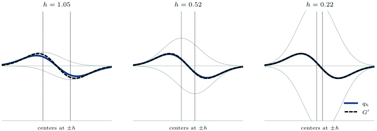
Figure 2. A two-neuron collision. The centered difference of two nearby Gaussians approaches a Gaussian derivative, while the signed amplitudes grow like 1/h The panels depict the visual story as the centers move closer together. Figure courtesy of Ziqian Li.
Now, choose a simple elliptic PDE whose exact solution is u=G'. On the whole line, for example, one may take
-u'' + u = f,
with f chosen accordingly. The PDE energy controls the H^1 error. Since
q_h converges to G' the neural states converge to the exact solution. However, the optimization problem over the two-neuron parametrization has no finite minimizer. If pushed toward exact minimization, the optimizer chases a boundary state of the realization class. Figure 3 summarizes the corresponding diagnostic contrast in a deliberately nonquantitative way; along the same training path, coordinate diagnostics may look unstable while state-space diagnostics show convergence.
What Should Be Monitored?
The example is elementary, but the lesson is not limited to Gaussians. Its value lies in the fact that it isolates—in the simplest possible form—a mechanism that can occur whenever nonlinear realization maps have non-closed images or poorly compact parameterizations. Many neural realization classes are nonlinear and non-closed, and their topology in parameter space can differ substantially from their topology in the physical function space. This is precisely where parameter escape and state convergence can coexist.
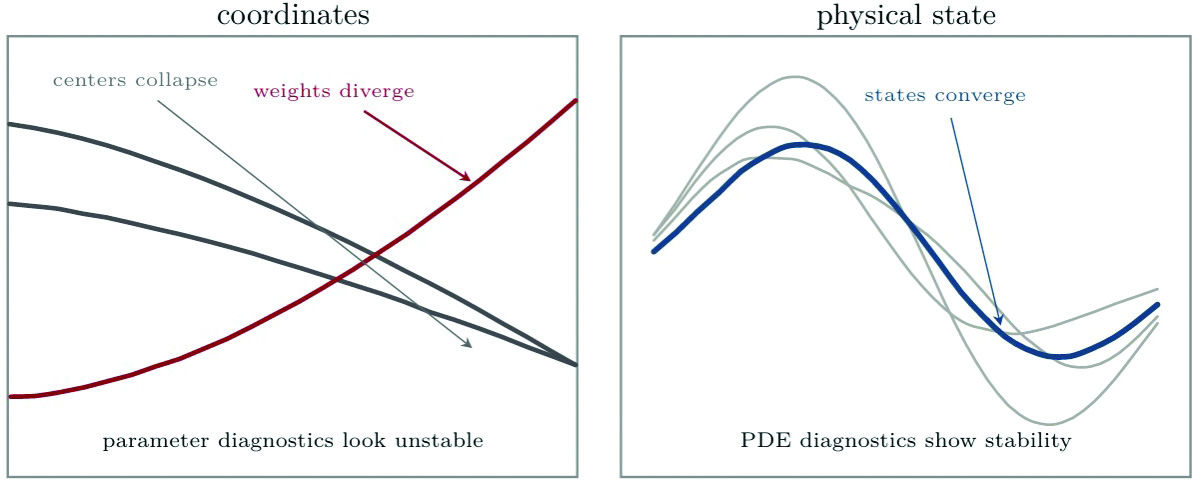
Figure 3. The same sequence can look unstable in coordinates and stable in state space. While not quantitative, this schematic illustrates the diagnostic distinction behind the coercivity gap. Figure courtesy of Ziqian Li.
For practitioners, the distinction changes what should be treated as evidence. Large parameter values observed during training may indicate a difficult representation or a poorly conditioned search, but it does not by itself confirm the accuracy of the PDE state. Conversely, a small training loss is most meaningful when it is connected to a stability estimate in the physical norm.
For energy methods like the deep Ritz method, the relevant question is whether the energy is coercive in the state norm. For residual methods such as PINNs, the question rests on whether the residual is measured in a norm that yields a PDE stability estimate. In both cases, the useful diagnostic is state accuracy—or a residual with a genuine stability meaning—rather than the mere boundedness of the coordinates.
This does not remove the importance of optimization, and initialization, training dynamics, conditioning, and regularization remain central practical issues. The coercivity gap simply warns that these issues should not be confused with the mathematical stability of the realized PDE state.
This perspective separates three questions that can be merged with classical discretizations. Does the loss control the physical state in the right norm? Is the neural parametrization compact or well conditioned? Can the training algorithm reach the relevant energy level? A successful computation requires attention to all three, but they are not the same question.
Conclusion
The coercivity gap is the failure of state-space coercivity to imply parameter-space compactness; it does not invalidate stability or coercivity as guiding ideas for numerical analysis. Instead, it affirms that these ideas operate after the realization map in neural PDE solvers, on the physical state that the differential equation sees.
Understanding this distinction can make numerical evidence easier to interpret. Neural PDE solvers optimize in parameter space but are judged in state space. Sometimes good numerical states are reached through deteriorating coordinates.
The broader challenge is to build a numerical analysis of neural PDE solvers that can clearly distinguish between approximation in state space, compactness in parameter space, and success of the training dynamics. While classical methods often hide this distinction because their coordinates and states are tightly coupled, neural methods expose it. Turning this exposure into reliable diagnostics, robust algorithms, and high-fidelity solvers is one of the mathematical tasks ahead.
References
Cite this work:
Zuazua, E. (2026). Good Solutions, Bad Coordinates: The Coercivity Gap in Neural Partial Differential Equation Solvers. SIAM News, 59(7). arXiv: 2510.03303, FAU CRIS
This article has been published on SIAM News:
https://www.siam.org/publications/siam-news/articles/good-solutions-bad-coordinates-the-coercivity-gap-in-neural-partial-differential-equation-solvers