Corrosion at the Junction

Singular limits and learned shortcuts for galvanic corrosion: a visual, runnable tour of two FAU × Schaeffler papers.

Author: Daniel Fernández

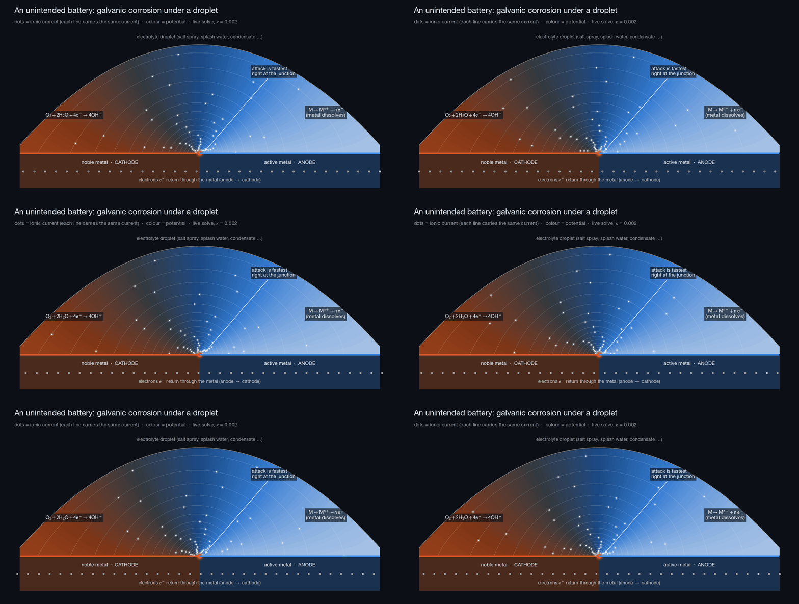
The electrolyte potential tears into a step at the cathode–anode junction as the conductivity parameter κ decreases

Why it matters

Corrosion is expensive. Its global cost is estimated at US$ 2.5 trillion per year, about 3.4 % of world GDP. An estimated 15–35 % of that could be avoided with existing corrosion-control practice (NACE IMPACT study, 2016).
Galvanic corrosion comes with multi-material design. Wherever two different metals share an electrolyte (housings and bearing seats, fasteners and joints, scratched or cut coatings), they form a battery that dissolves the more active metal. Lightweight, electrified products create ever more such contacts. Tests take weeks, field exposure takes years, and so the decisions made early in design rely on simulation.
The low-conductivity regime matters most. In humid air, condensation, rain and splash water, the corrosion current cannot spread out and concentrates at every cathode–anode junction. In this regime half of the metal loss can occur within about 50 µm of the junction. This is also where simulations become singular: stiff boundary laws, jumps, and layers of width ∝ κ that defeat uniform meshes and slow down solvers. The two papers below analyse exactly this regime [1] and turn it into a speed-up [2].

Our interactive notebook rebuilds both papers with a compact finite-element solver (under 200 lines), reproduces their archived numbers, and visualises every result. Everything runs top to bottom in about four minutes on a laptop.

	Paper	Code
[1]	D. Fernández, Singular limit phenomenon in a nonlinear elliptic model arising in electrochemistry, arXiv:2606.20619	singular-limit-corrosion
[2]	D. Fernández, D. Penk, D. Riedelbauch, Selective boundary condition reduction via learned error gating, arXiv:2609.08461	learning-boundary-condition

Galvanic corrosion is a boundary phenomenon

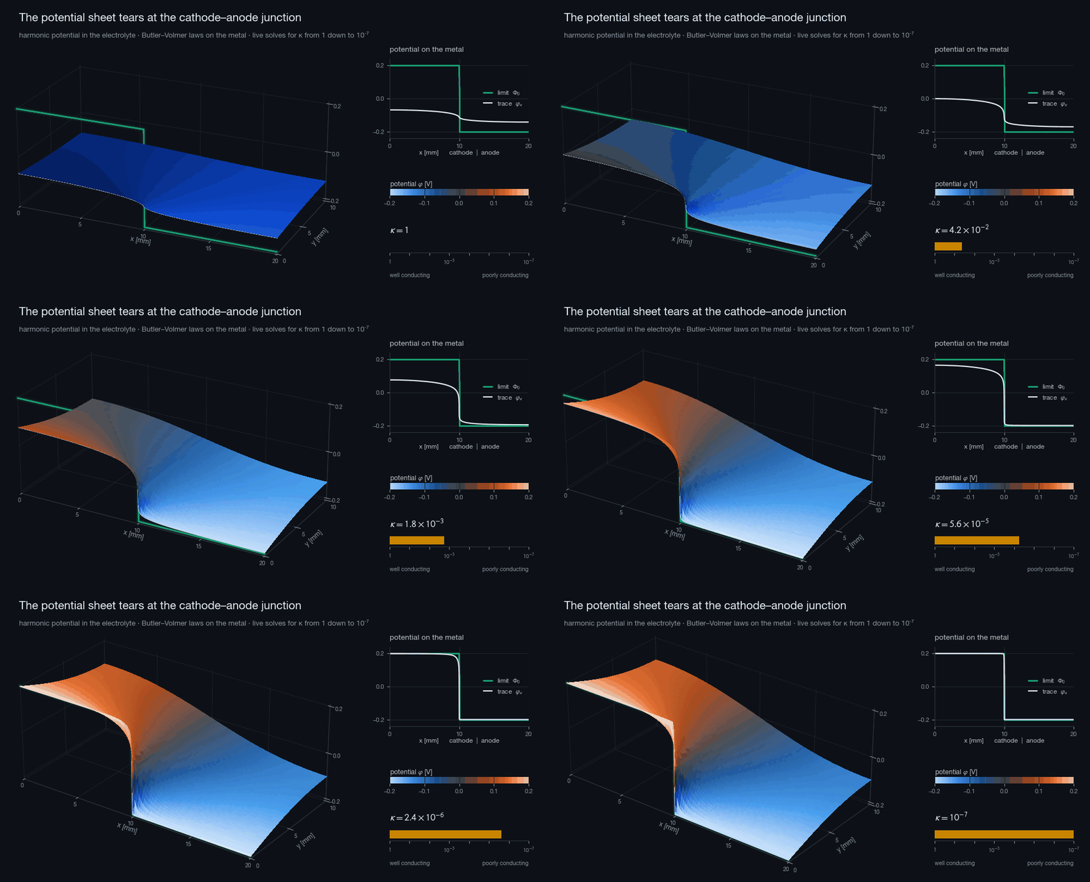
The potential is harmonic in the electrolyte, and each metal surface follows an exponential Butler–Volmer law. A single dimensionless conductivity κ (electrolyte conductance relative to the surface kinetics) decides how the corrosion current is distributed.

Ionic current lines under a salt-water droplet on a bimetallic joint, crowding into the junction

The singular limit κ → 0 [1]

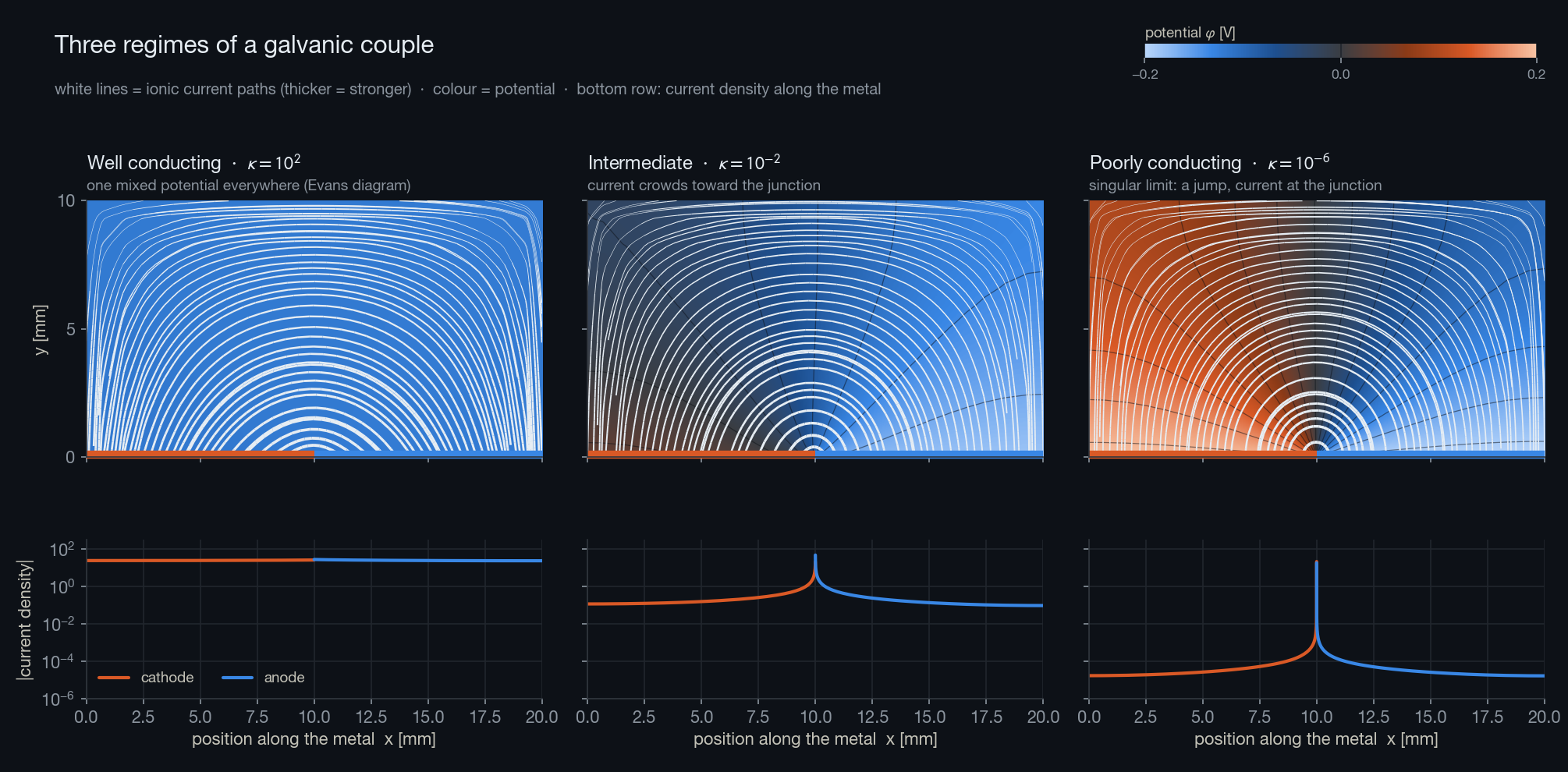
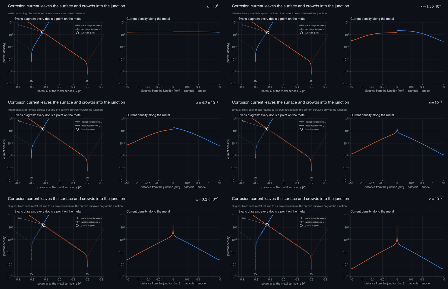
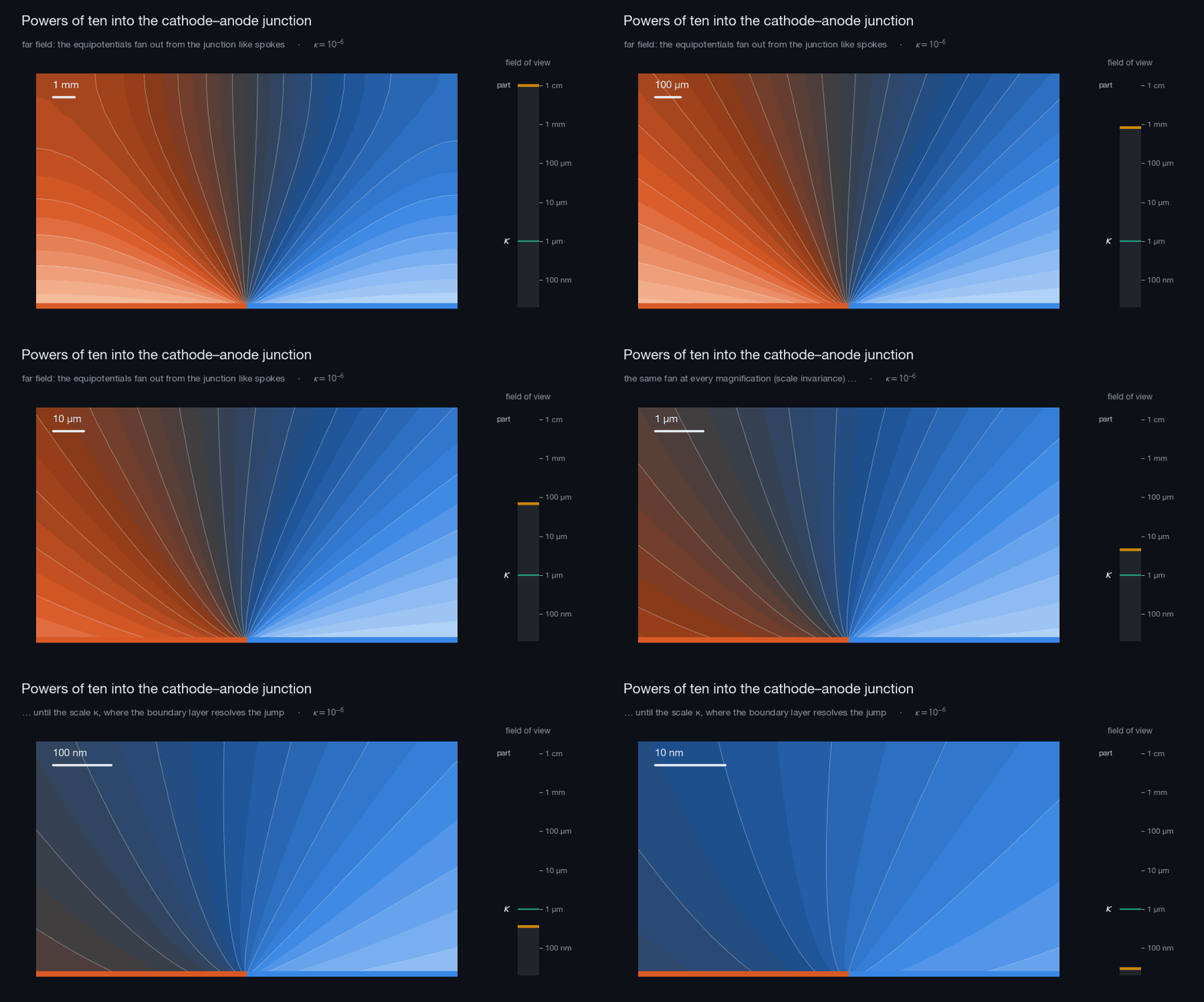
Potential and current paths for κ = 10², 10⁻² and 10⁻⁶

From uniform Evans-diagram behaviour (κ = 10²) to the singular limit (κ = 10⁻⁶): the potential on the metal snaps to a step, and the current collapses into the junction.

Every surface point slides along its Butler–Volmer curve	Powers of ten into the junction

Theorem 2.1 / Corollary 2.1. The surface potential converges to the step, and the interior converges to its mixed harmonic extension. Fitted live rates: boundary slope 1.07 (theory 1), interior slope 0.81 (proved bound ½).
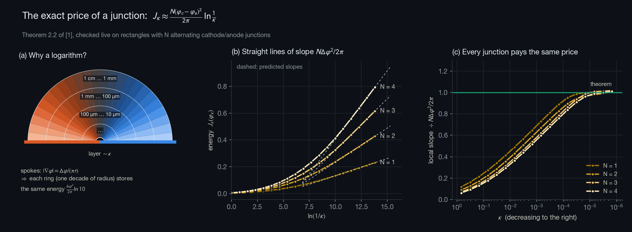
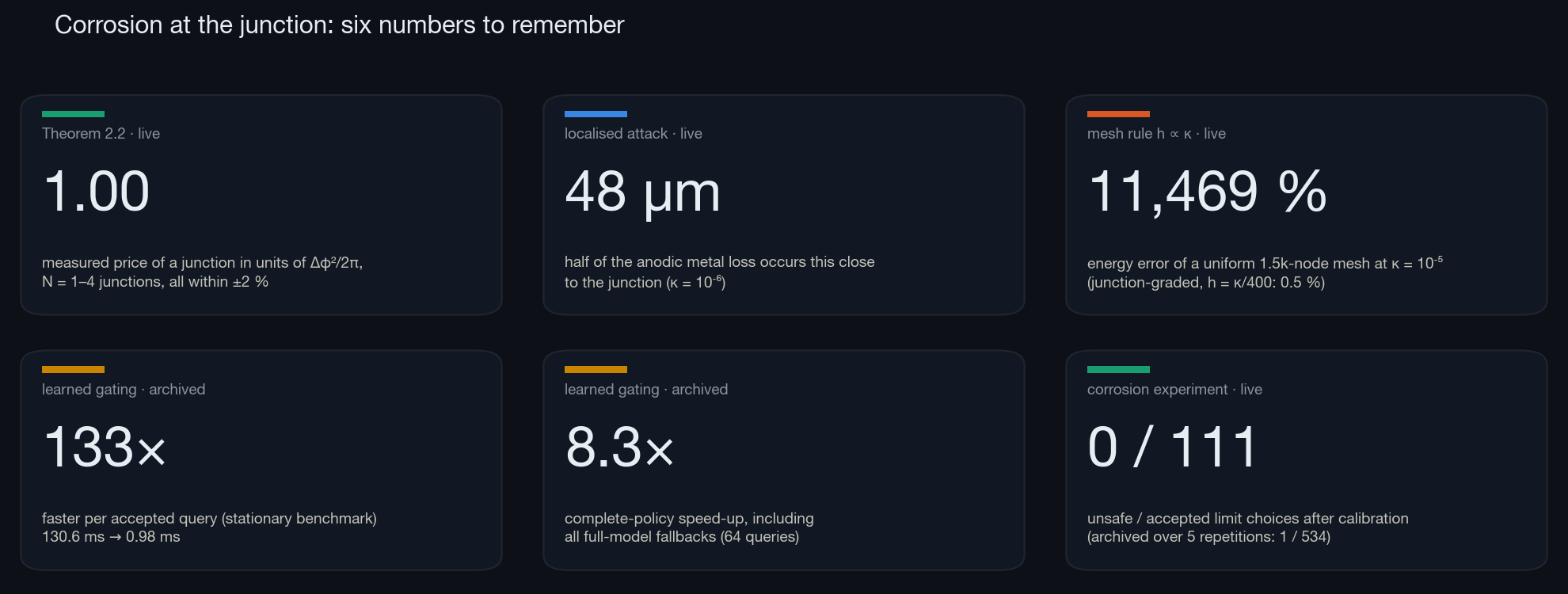
Theorem 2.2. The energy grows like $\frac{N(\varphi_c-\varphi_a)^2}{2\pi}\ln\frac1\kappa$ , one universal price per junction. The notebook measures it for N = 1–4 junctions to within ±2 %.
Localised attack. Half of the anodic metal loss occurs within 4.8 mm of the junction at κ = 10², but within 48 µm at κ = 10⁻⁶.
Mesh rule. Resolve the layer, not the part. Junction-graded meshes with
$h_{\min}\propto\kappa$ stay accurate as κ → 0 (0.5 % energy error at κ = 10⁻⁵), while a uniform mesh with a similar node budget is off by more than 11,000%.

Energy law: J grows like N Δφ²/2π ln(1/κ)

Learned error gating

Many-query studies need the corrosion model hundreds of times. The Dirichlet limit is one reusable linear solve, but is it accurate enough for this case? A small network predicts the domain and boundary errors of the cheap model before solving. The limit is used only when both predicted errors meet the tolerances, and otherwise the full nonlinear model runs.

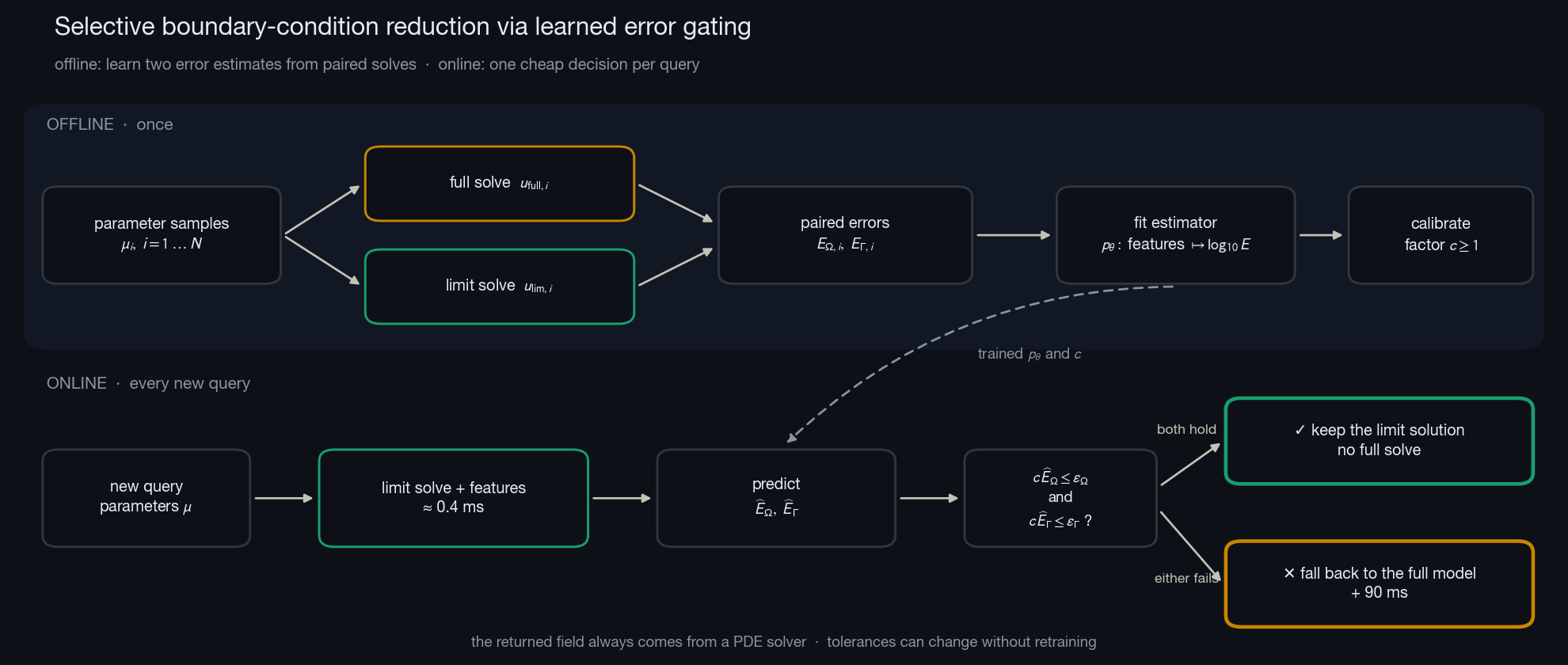
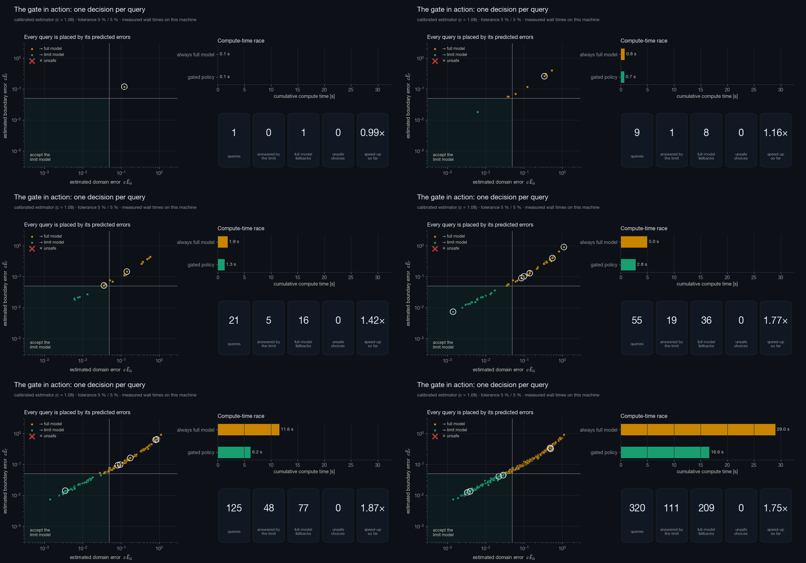
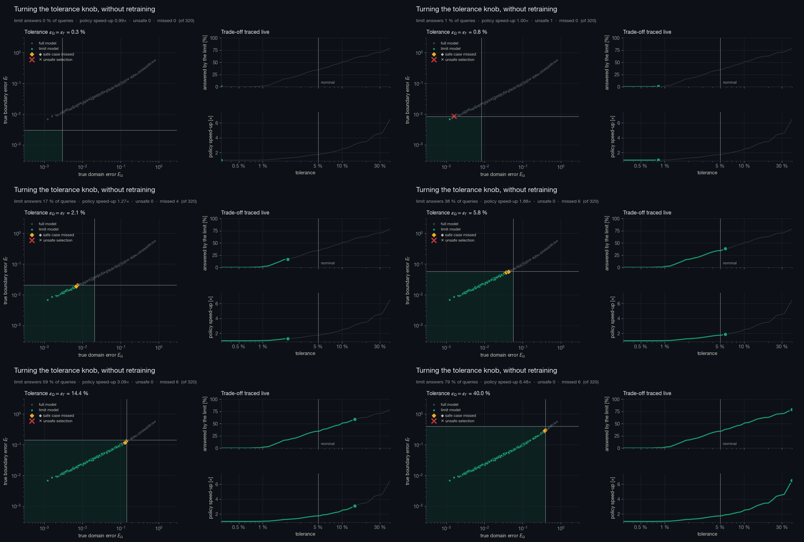
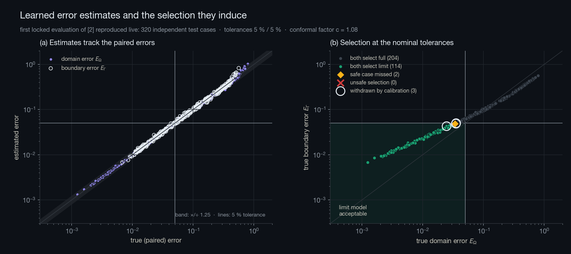
Offline training on paired solves and online gating of each query

The notebook reproduces the paper’s corrosion experiment live (same seeds, mesh, features, and estimator). It matches the archived spot check to seven digits, and on the first locked evaluation (320 cases, 5 % tolerances) the calibrated gate makes 0 unsafe choices in 111 limit uses, as in the paper. On a laptop an accepted query is ≈ 200× cheaper (about 0.4 ms instead of 90 ms):

The gate in action	The tolerance knob (no retraining)

Estimated versus paired errors and the decision plane

Six numbers to remember

Summary tiles

Run it

python -m pip install numpy scipy matplotlib scikit-learn pillow jupyterlab jupyter lab corrosion_at_the_junction.ipynb # then: Run ▸ Run All Cells

Set FAST = True in the setup cell for a ~2-minute preview. Figures and GIFs are written to assets/, and the paired dataset of Part III is cached in .cache/.

Folder content
`corrosion_at_the_junction.ipynb`	the guided tour (Parts I–IV, executed, with outputs)
`assets/`	every figure (PNG) and animation (GIF) produced by the notebook
`README.md`	project overview (this page)

Research by FAU Erlangen-Nürnberg (Chair for Dynamics, Control, Machine Learning and Numerics, Alexander von Humboldt Professorship) and Schaeffler Technologies AG & Co. KG. Both works were funded by Schaeffler Technologies AG & Co. KG.