
Author: Bo You
Every forecast begins from an estimated state rather than nature’s exact one. Weather stations leave spatial gaps, ocean sensors sample only a small fraction of the water column, and experiments with multiphase fluids cannot reveal every velocity and concentration at every point. Even a highly accurate numerical solver may therefore evolve the wrong initial state and gradually drift away from the physical system that it is meant to represent.
Data assimilation closes this gap by combining a mathematical model with incoming observations. One particularly transparent approach is continuous data assimilation, also known as the Azouani–Olson–Titi (AOT) algorithm [1]. It runs a second copy of the model from an arbitrary initial guess and continually nudges the observed features of that copy toward the data. For many dissipative systems, sufficiently informative measurements and an appropriately chosen nudging strength cause the estimated state to forget its initial error and synchronize with the reference trajectory.
The mechanism becomes visible in a two-fluid computation: an estimate that begins from random fields can recover the evolving interface of a square-shaped inclusion as surface tension rounds it into a circle. In joint work with Qing Xia [4], we extended the continuous data assimilation framework to the two-dimensional Cahn–Hilliard–Navier–Stokes system and established exponential synchronization under suitable conditions on the observation resolution and nudging parameters. The numerical experiment below illustrates this result. It also clarifies what the algorithm can and cannot do: AOT primarily corrects uncertainty in the evolving state; it is not, by itself, a universal remedy for incorrect governing equations or persistent structural model bias.
A Feedback Loop Between Equations and Data
At a schematic level, suppose that the unavailable reference state u(t) evolves according to
\frac{du}{dt}=F(u), \qquad (1)
where F represents the governing dynamics. Instead of attempting to reconstruct the full initial state
directly, the AOT algorithm evolves an estimate v(t) according to
\frac{dv}{dt}=F(v)+\mu\bigl(I_h(u)-I_h(v)\bigr), \qquad v(0)=v_0.
Here, v0 can be an arbitrary initial guess, Ih(u) denotes the information that the sensors actually observe, and Ih(v) is the same information extracted from the simulation. Depending on the application, Ih might represent values at sensor locations, local averages, finite-volume measurements, or a projection onto a set of large-scale Fourier modes. The parameter h characterizes the observation resolution, while the positive gain μ controls the strength of the feedback.
Equation (2) has a simple interpretation. The model term F (v) advances the estimate according to the known physics. The feedback term compares predicted and measured features and pushes the estimate in the direction that reduces their mismatch. Once those features agree, the correction vanishes. Meanwhile, the model transports the information from observed scales and locations into parts of the state that are not directly measured.
Equation (2) summarizes the feedback principle in compact form. In the coupled CHNS application, analogous correction terms act on the observed phase and velocity components.
The observation spacing and the nudging gain must be chosen together. If the measurements are too coarse, dynamically important structures can remain unseen; simply increasing μ cannot recover information that the sensors never capture. Mathematical analysis of the error v − u balances the model’s dissipation, the feedback strength, and the approximation properties of Ih. In the noiseless settings analyzed in [1, 3, 4], the error decays exponentially in time when this balance holds. In a discrete-observation variant with bounded measurement errors, the long-time discrepancy is instead controlled by the noise level [2]. After synchronization, one may either continue assimilating data or usev(T ) as the initial state for a forecast beyond the final observation time T .
Watching Synchronization Happen
To illustrate this mechanism, consider the two-dimensional Cahn–Hilliard–Navier–Stokes (CHNS) system, which couples the motion of an incompressible fluid to the separation of two phases [4]. A phase-field variable distinguishes the two fluids, and its zero contour marks their interface. Surface tension favors shorter interfaces, so an isolated square-shaped region naturally rounds into a circle (see Figure 1).
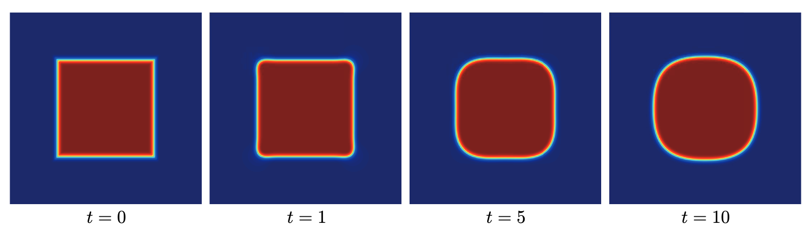
Figure 1: The reference CHNS trajectory. Surface tension transforms the initial square-shaped inclusion into a circle. Figure courtesy of the author; numerical experiment reported in [4].
This computation is a synthetic twin experiment: the reference trajectory and the partial observations are generated by the same CHNS model. Both the assimilated and unnudged simulations begin from the same randomly generated phase and velocity fields, so that the comparison isolates the effect of AOT feedback. The reference calculation uses a 256 × 256 grid on the square domain [−1, 1]2, and the observations are sampled on a coarser grid comprising 16,384 nudging locations—one quarter of the computational grid. These sampled phase and velocity data enter the corresponding feedback terms in the assimilated CHNS system. Figure 2 compares the resulting trajectories. The upper row includes AOT feedback from the reference observations; the lower row evolves under the original CHNS dynamics without nudging. The nudged solution progressively organizes itself around the correct interface and reaches the target circle, whereas the unnudged solution retains a very different multiphase pattern.
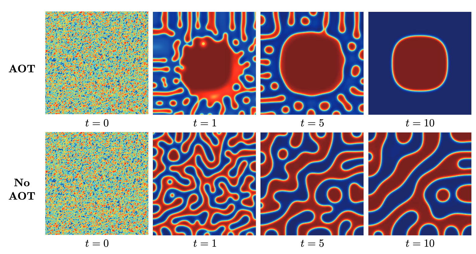
Figure 2: Two simulations from the same random initial state. The AOT-nudged solution (top) synchronizes with the square-to-circle reference trajectory, while the CHNS solution without AOT feedback (bottom) does not. Figure courtesy of the author; numerical experiment reported in [4].
The zero contours in Figure 3 provide a sharper comparison. At first, the interface of the assimilated state bears little resemblance to the observed one. The mismatch then contracts, and the two contours are nearly indistinguishable by t = 10. The pictures do not replace a convergence proof, but they make its central mechanism tangible: feedback suppresses errors on the observed scales, and dissipation prevents unresolved errors from persisting indefinitely.
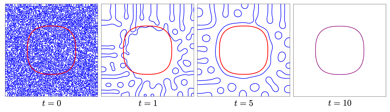
Figure 3: Zero-contour comparison of the assimilated interface (blue) and the synthetic reference interface (red). Their near coincidence at t = 10 indicates synchronization. Figure courtesy of the author; numerical experiment reported in [4].
What the Guarantee Does—and Does Not—Say
Continuous nudging is appealing for high-dimensional partial differential equations because the correction enters directly into the evolution law and only requires observed features rather than the complete state. Related schemes can also accommodate measurements that arrive at discrete times, provided that the time between observations is sufficiently short and the resolved scales are sufficiently informative [2]. These properties make the framework relevant to ocean and weather prediction, environmental monitoring, materials simulation, and physics-based digital twins.
The assumptions behind the guarantee are just as important as the conclusion. Partial or poorly placed observations may miss active structures, noisy measurements impose an accuracy floor, and biased observations may steer the estimate away from the desired trajectory. Most importantly, the dynamicsF must capture the essential physical mechanisms. If the equations contain persistent bias or omit important processes, state nudging alone cannot identify and repair that structural error. Such situations call for simultaneous state and parameter estimation, explicit model-error representations, or hybrid physics–data approaches.
The broader lesson is therefore not that observations should replace physical models, or that models can make observations unnecessary. Their strengths are complementary: equations propagate information through space and time, while observations prevent the simulated trajectory from drifting away from reality. Continuous data assimilation turns that partnership into a feedback loop, and rigorous mathematics specifies when the loop is strong enough to yield a reliable reconstruction.
References
1. Azouani, A., Olson, E., & Titi, E. S. (2014). Continuous data assimilation using general interpolant
observables. Journal of Nonlinear Science, 24 (2), 277–304.
2. You, B. (2024a). A discrete data assimilation algorithm for the three-dimensional planetary geostrophic equations of large-scale ocean circulation. Journal of Dynamics and Differential Equations, 36 (2), 1591–1615.
3. You, B. (2024b). Continuous data assimilation for the three-dimensional planetary geostrophic equations of large-scale ocean circulation. Zeitschrift f ̈ur Angewandte Mathematik und Physik, 75, Article 147.
4. You, B., & Xia, Q. (2022). Continuous data assimilation algorithm for the two-dimensional Cahn–Hilliard–Navier–Stokes system. Applied Mathematics & Optimization, 85 (2), Article 5.About the AuthorBo You is with the School of Mathematics and Statistics at Xi’an Jiaotong University.
About the Author
Bo You is with the School of Mathematics and Statistics at Xi’an Jiaotong University. Research interests include partial differential equations and data assimilation for geophysical and multiphase-flow models.