Author: Antonio Álvarez-López
A model can remember every example in its training set and still fail on the next one. This familiar tension between interpolation and generalization becomes particularly interesting for neural ordinary differential equations (neural ODEs), where a prediction is produced by continuously moving the input through space. If the model can steer every training point to its prescribed target, have we learned anything about what happens to points that were never seen during training?
In our recent work with Lorenzo Liverani and Enrique Zuazua [3], we approach this question from control theory. Control-theoretic approaches to neural ODEs have been developed in [6], while quantitative questions of interpolation and architecture have also been studied in [7]. The basic idea is to view a neural ODE as a dynamical system whose parameters act as controls. This viewpoint makes interpolation a geometric routing problem: one vector field must move many initial points to many prescribed destinations at the same time. The key step is then to strengthen this pointwise picture. Instead of asking the flow to move only the training samples, we ask it to move whole regions around them. That stronger property provides a direct route from expressivity to quantitative generalization.
Learning as a flow
The idea of describing learning through continuous dynamical systems was proposed explicitly in [1], and neural ODEs turned this viewpoint into a trainable continuous-depth architecture [2]. Starting from an inputx(0) = x0, the state evolves according to an equation of the form
\dot x(t)=v_\theta(t,x(t)),
and the prediction is the final position x(T ). In the architecture we study, the vector field is generated by a shallow ReLU network,
\dot x(t)=\sum_{j=1}^{p} w_j\,\big(a_j\!\cdot x(t)+b_j t+c_j\big)_+.
The spatial weights w_j and a_j are fixed in time; the only explicit time dependence comes from the affine term b_jt+c_j. We call this a \emph{semi-autonomous neural ODE}. Equivalently, one can think of a standard time-independent network acting on the augmented variable (x,t).
This is a small departure from a fully autonomous system, but it has a surprisingly large effect. Geometrically, each ReLU introduces an activation hyperplane. In an autonomous model those hyperplanes are fixed in space. Here they can translate as time passes. This moving geometry gives the flow a way to schedule different parts of the transport without changing all parameters independently at every instant.
The first question is whether this restricted architecture is expressive enough even at the level of the training data. The answer is yes: for any admissible dataset of N distinct input–target pairs in dimension d\geq2, one can construct a semi-autonomous neural ODE that maps every input \emph{exactly} to its target. A width of 2N is sufficient in our construction.
Thus, even with this very limited form of time dependence, exact interpolation is possible. But exact interpolation is only the beginning. The left panel of Figure~\ref{fig:process} illustrates this first, purely pointwise, level of control: the observed samples can be sent exactly to their prescribed destinations, while nothing is yet required of the surrounding space.
From points to cells
Suppose that a training point $x_i$ is mapped perfectly to its label $y_i$. A nearby unseen point may nevertheless be sent somewhere completely different. Point interpolation therefore says almost nothing by itself about the population error. To connect the two, we introduce the stronger requirement of \emph{simultaneous cell controllability}.
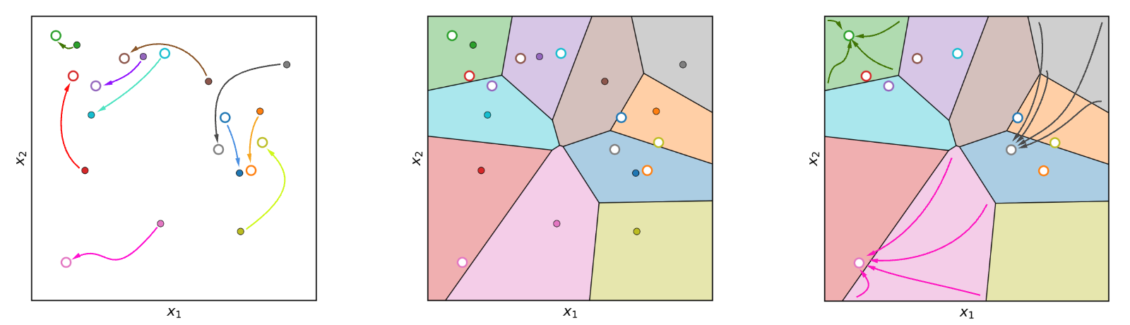
Figure 1: From interpolation to generalization. Left: the flow sends the observed inputs to their prescribed targets.Center: the input domain is divided into regions associated with the data, here a Voronoi partition. Right: rather than
controlling only isolated samples, the flow compresses entire cells toward the corresponding targets. This regional version of controllability is the mechanism used to obtain generalization bounds. Source: [3].
Imagine dividing the input space into disjoint cells $A_1,\ldots,A_K$. For each cell we choose a target $r_k$. Cell controllability asks for a single neural ODE flow that sends \emph{every point} of $A_k$ into a small ball around $r_k$, simultaneously for all cells. Figure~\ref{fig:process} shows the progression from interpolation to this stronger form of control. The left panel contains the original pointwise problem; the center panel replaces isolated samples by a partition of the domain; and the right panel shows the desired outcome, in which each entire cell is transported close to its representative target.
The distinction is important. Moving finitely many particles leaves a great deal of empty space between them. Moving macroscopic regions is much more restrictive: the flow must coordinate infinitely many initial conditions at once and cannot simply let trajectories pass through one another. Nevertheless, we prove constructively that semi-autonomous neural ODEs can perform this task for arbitrary finite families of disjoint compact convex cells, to any prescribed accuracy, provided the width is large enough.
The proof has a simple geometric picture. First, each input cell is compressed into a very small packet. These packets are then transported along separate corridors toward their destinations. Finally, the resulting smooth steering field is approximated by the ReLU vector field of the neural ODE. The quantitative estimates are conservative—the required width can become very large when cells are numerous or lie very close to one another—but the conclusion is qualitative and robust: the architecture can control regions, not just samples.
A classical estimator hidden inside the flow
Why does controlling cells help with generalization? Because many classical statistical estimators already work cell by cell.
A histogram estimator partitions the input domain into boxes and assigns one value to each occupied box. A nearest-neighbor estimator uses a Voronoi tessellation and assigns to every point the label of its closest sample. Both are piecewise-constant rules. They are crude compared with a neural network, but their statistical behavior is classical and well understood \cite{Stone1982,Gyorfi2002}. Figure~\ref{fig:nonparam} shows these two constructions side by side: a regular grid for the histogram and a data-dependent Voronoi partition for nearest neighbors.
Cell controllability lets us embed precisely this idea into the neural ODE. We first build a standard nonparametric estimator from the data. We then construct a flow that sends each cell close to the value selected by that estimator. In the language of Figure~\ref{fig:nonparam}, the neural ODE is asked to reproduce the piecewise-constant map represented by the center or right panel. The total prediction error separates into two pieces: the usual statistical error of the nonparametric method, plus the error incurred when the neural ODE realizes it. If the network is wide enough, the second term can be made smaller than the first.
This gives explicit population-risk guarantees. For an $\alpha$-H\”older target in $d$ dimensions, the construction recovers the familiar rates
N^{-\frac{2\alpha}{2\alpha+d}} \qquad\text{and}\qquad \left(\frac{\log N}{N}\right)^{\frac{2\alpha}{d}}
for histogram and nearest-neighbor constructions, respectively. The main point is not that a neural ODE should literally behave like a histogram in practice. Rather, these estimators provide a certificate: the model class is rich enough to contain data-dependent predictors whose true error provably vanishes at a quantitative rate.
This is a different perspective from standard generalization bounds based on uniform control over a parameterized model class, as developed for neural ODEs and deep residual networks in \cite{Marion2023Generalization}. Instead of controlling the worst possible model inside a parameter class, we explicitly build one particular flow adapted to the observed data and compare it with a statistically understood benchmark. Overparameterization is therefore not treated only as a liability to be bounded; sufficient width is also a resource that makes the desired transport possible.
There is an important caveat. Our current width estimates are worst-case guarantees and can grow super-polynomially with the sample size because increasingly fine partitions create narrow geometric corridors. We do not claim that such widths are necessary. In fact, our numerical experiments suggest the opposite: trained models often match or outperform the nonparametric baselines with widths far below those required by the proof. Closing this gap is one of the main quantitative questions left open by the theory.
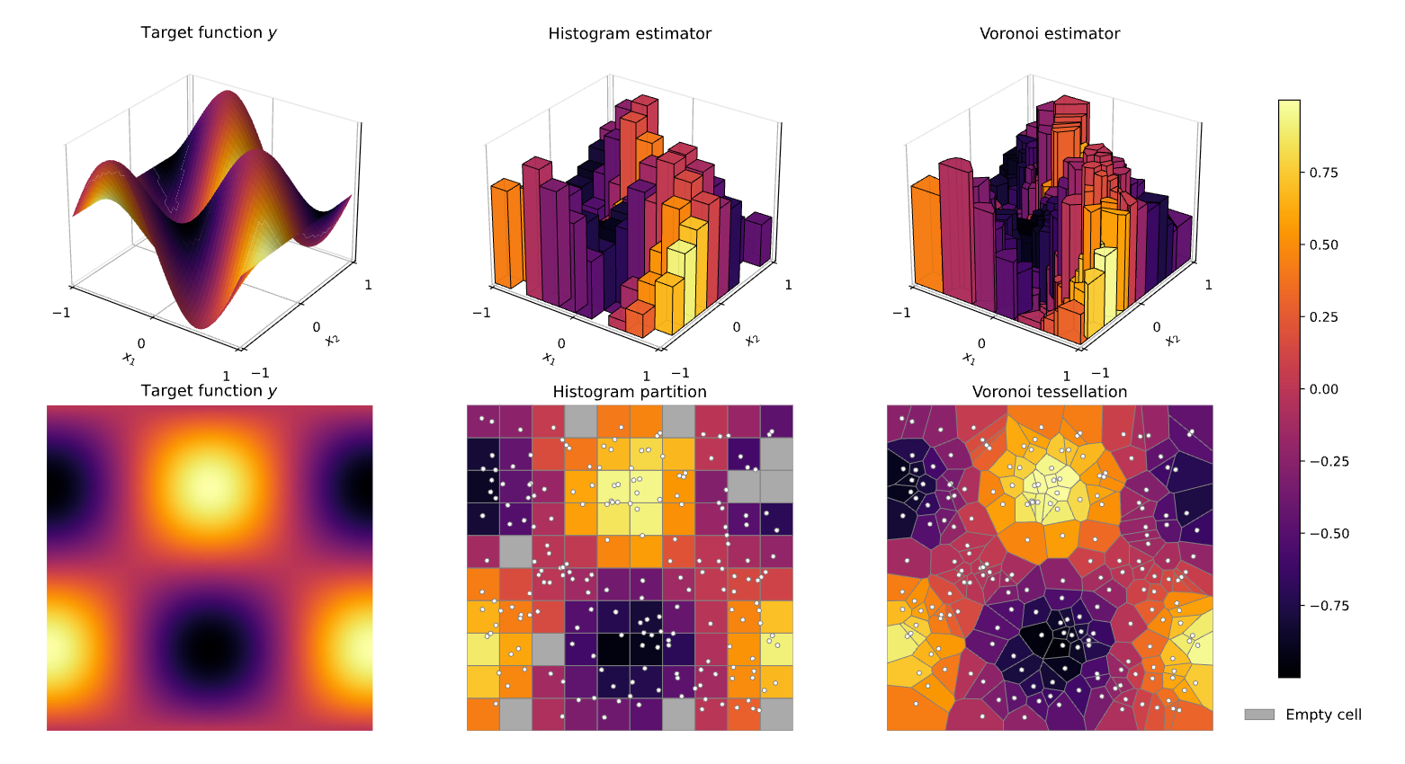
Figure 2: Two classical nonparametric approximations used as statistical benchmarks. Left: the target map. Center: a histogram approximation, constant on a regular grid. Right: a nearest-neighbor approximation, constant on Voronoi cells. Simultaneous cell controllability allows a semi-autonomous neural ODE to reproduce these piecewise-constant rules up to a small realization error. Source: [3].
Why a little time dependence matters
The role of the term $b_jt$ becomes clear when we remove it. In a fully autonomous neural ODE, the vector field is fixed once and for all. Such systems can still be very expressive. In particular, we show that a two-layer autonomous model can exactly interpolate finite datasets under a natural geometric nondegeneracy condition.
Yet point interpolation and cell routing are different problems. An autonomous flow cannot make two trajectories cross: uniqueness of the ODE forbids it. For isolated points, paths can often bend around one another. Entire regions do not have that freedom. When several cells are interlaced and must be sent to different destinations, the required transport may be topologically incompatible with a single autonomous deformation.
A simple checkerboard experiment makes this visible. Adjacent squares are assigned alternately to two distant targets. As the checkerboard becomes finer, the two classes are increasingly interwoven. Figure~\ref{fig:checkerboard} shows a representative case. Reading from left to right, one sees the initial checkerboard, the two target locations, and the outputs produced by the semi-autonomous and autonomous models. We train the two models with essentially the same number of parameters. The time-dependent model can schedule the motion and separate the classes, whereas the autonomous output becomes progressively entangled.
This does not mean that time dependence is universally necessary for learning. The conclusion is more specific: for the generalization mechanism studied here—routing whole cells so as to realize local statistical estimators—autonomous flows face obstructions that disappear once even a simple time-dependence is introduced.
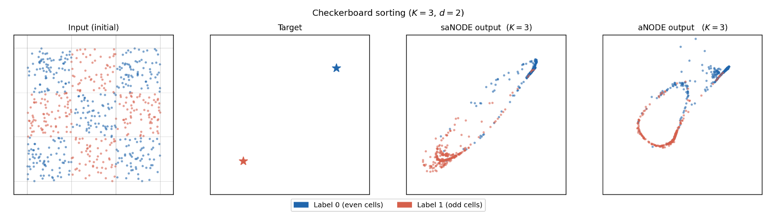
Figure 3: Checkerboard sorting at resolution K = 3. From left to right: input data, target assignment, output of the semiautonomous neural ODE, and output of a parameter-matched autonomous neural ODE. Explicit time dependence provides an additional space–time degree of freedom that allows the model to resolve the interlaced regions. Source: [3].
From expressivity to generalization
Control theory is often used to ask whether a dynamical system can reach a desired state. In learning, that question has usually been translated into interpolation: can one set of parameters steer all training samples to their labels? Our results suggest that the more relevant object may be a stronger, regional form of controllability. Generalization depends not only on where the observed points go, but on what the model does in the space between them. Semi-autonomous neural ODEs provide a particularly transparent setting in which these two levels coexist. They can interpolate finite data exactly, control entire input cells, and thereby emulate classical estimators with known statistical rates. At the same time, comparing them with autonomous models isolates a concrete architectural feature—explicit time dependence—that changes what the flow can do geometrically. The broader message is that expressivity and generalization need not be studied as separate phenomena. For flow-based models, the geometry of controllability can connect them directly: first understand how information can be transported through space, then use that transport to reproduce estimators whose statistical behavior is already known. In this sense, the path from training data to unseen data is itself a dynamical object.
References
[1] W. E, “A Proposal on Machine Learning via Dynamical Systems,” Communications in Mathematics and Statistics, 5(1), 1–11, 2017. doi: 10.1007/s40304-017-0103-z.[2] R. T. Q. Chen, Y. Rubanova, J. Bettencourt, and D. Duvenaud, “Neural Ordinary Differential Equations,”Advances in Neural Information Processing Systems, 31, 2018.
[3] A. Álvarez-López, L. Liverani, and E. Zuazua, “Constructive interpolation and generalization rates for neural ODEs: a control perspective,” preprint, 2026.
[4] C. J. Stone, “Optimal global rates of convergence for nonparametric regression,” The Annals of Statistics, 10(4), 1040–1053, 1982.
[5] L. Györfi, M. Kohler, A. Krzyżak, and H. Walk, A Distribution-Free Theory of Nonparametric Regression, Springer, 2002.
[6] D. Ruiz-Balet and E. Zuazua, “Neural ODE Control for Classification, Approximation, and Transport,” SIAM Review, 65(3), 735–773, 2023. doi: 10.1137/21M1411433.
[7] A. Álvarez-López, A. Hadj Slimane, and E. Zuazua, “Interplay between depth and width for interpolation in neural ODEs,” Neural Networks, 180, 106640, 2024. doi: 10.1016/j.neunet.2024.106640.
[8] P. Marion, “Generalization Bounds for Neural Ordinary Differential Equations and Deep Residual Networks,” Advances in Neural Information Processing Systems, 36, 48918–48938, 2023.