
Authors: Xinyu Cheng, Yunzhang Li, Weiran Xiong, Enrique Zuazua
Partial differential equations (PDEs) describe how quantities evolve in space and time, with applications in fluid dynamics, finance, control, physics, and biology. What happens when a PDE has 100 spatial variables? Even a very coarse grid with only 10 points in each direction would contain 10^{100} points, far beyond any realistic computation.
One possible strategy is to avoid constructing the grid altogether and instead represent the PDE through an associated stochastic system. Through the nonlinear Feynman–Kac formula, suitable nonlinear parabolic PDEs can be represented by forward–backward stochastic differential equations (FBSDEs). This representation replaces approximation across the entire spatial domain with computations along random trajectories.
Although the FBSDE representation avoids constructing a full spatial grid, it introduces unknown high-dimensional functions that determine the backward variables Y and Z from the simulated state. Neural networks provide flexible approximations of these functions, while Monte Carlo simulation generates training samples directly from the stochastic dynamics. The resulting loss can be minimized by stochastic gradient methods, allowing the computation to focus on solution values along relevant trajectories rather than resolving the entire spatial domain. Deep learning does not remove every difficulty associated with high dimension, but it can make these pathwise approximation problems computationally tractable. A seminal development in this direction was the deep BSDE method [4], which has since inspired a broad range of related approaches; see, for example, [1, 5, 6, 9].
The effectiveness of these methods depends strongly on the structure of the underlying system. For fully coupled FBSDEs, the forward trajectories depend on the trainable parameters, creating an unstable feedback loop between the forward simulation and the backward approximation. This may lead to poor convergence or numerical instability, particularly under strong coupling or over long time horizons.
In recent work, we introduced the deep truncated FBSDE method for high-dimensional quasilinear PDEs and fully coupled FBSDEs [2]. The method reduces the unstable feedback between neural-network parameters and simulated forward paths, while pathwise training signals improve optimization over long time horizons. It is designed for strongly coupled systems and degenerate convection-dominated equations. Our numerical examples include a nearly inviscid Burgers equation before, near, and after shock formation, as well as a 100-dimensional quasilinear problem.
The deep truncated FBSDE method
For a broad class of quasilinear parabolic PDEs, the nonlinear Feynman–Kac [8] connects the PDE solution with an associated fully coupled FBSDE. The forward process X describes the evolution of the state, while the backward processes Y and Z carry information from the terminal condition backward in time. The system is fully coupled because the forward dynamics depend on the backward variables, which in turn depend on the forward state. Under suitable conditions, the connection to the PDE solution u is given by
Y_t=u(t,X_t), \qquad Z_t=D_xu(t,X_t)\,\sigma\bigl(t,X_t,u(t,X_t)\bigr). \qquad (1)
Thus, instead of approximating u throughout the entire spatial domain, one can simulate random trajectories and approximate the solution along those trajectories.
This grid-free representation is especially attractive in high dimension, but the forward–backward coupling also creates the main numerical difficulty that our method is designed to address.
The difficulty is that a neural approximation with parameters \Theta generates parameter-dependent paths X(\Theta).
An inaccurate approximation of (Y,Z) distorts the forward trajectories, and the next parameter update is then computed on these distorted paths.
A terminal loss may even decrease by moving X_T(\Theta), rather than by improving the backward approximation.
This leads to the vicious cycle illustrated in Figure~\ref{fig:vicious_cycle}.
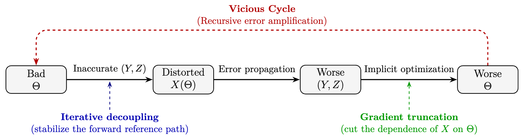
Figure 1: Instability mechanism in fully coupled FBSDE solvers. Figure courtesy of the authors.
Stabilizing the forward paths. We use gradient-truncated fictitious-play decoupling to separate the forward and backward components. At each iteration, the current numerical values of Y and Z still enter the forward dynamics, so the coupled structure is preserved. During backpropagation, however, a stop-gradient operation removes their parameter dependence through the simulated forward path. The backward equation is evaluated along a reference path constructed from previous forward iterates, and fictitious-play averaging reduces abrupt changes between consecutive reference paths.
Reconstructing Z from the neural solution. We introduce a neural reference process \widehat Y along the reference path and reconstruct Z from the spatial derivative of \widehat Y through the nonlinear Feynman–Kac relation (1). The reconstructed Z is then used throughout the simulated trajectory, yielding a global pathwise representation of the coupled dynamics.
Training along the entire trajectory. The training objective combines terminal matching along the current forward trajectory with a time-averaged consistency term between the simulated process Y and the neural reference process \widehat Y. The consistency term acts at intermediate times and creates local gradient shortcuts that do not rely solely on backpropagation from the terminal condition. It therefore provides a structural mechanism that can mitigate gradient vanishing over long time horizons.
Numerical illustrations
A nearly inviscid one-dimensional test. We first consider the viscous Burgers equation
\left\{ \begin{aligned} &u_t^\varepsilon+u^\varepsilon u_x^\varepsilon=\varepsilon u_{xx}^\varepsilon,\\ &u^\varepsilon(0,x)=\sin x. \qquad (2) \end{aligned} \right.
For the corresponding inviscid equation, the first shock forms at T_b=1; see [7].
We examine T=0.5,1.0,1.5, representing the pre-shock, shock-formation, and post-shock regimes, with \varepsilon=10^{-2},10^{-5},10^{-8}.
After time reversal, nonlinear transport is incorporated into the forward drift of a coupled FBSDE. This formulation represents the viscous solution for each \varepsilon>0 while avoiding the singular factor \varepsilon^{-1/2} that appears in the backward generator of the standard decoupled formulation. Figure 2 compares the resulting vanishing-viscosity approximations with the entropy solution of the inviscid equation. The discrepancy therefore includes both the vanishing-viscosity and numerical approximation errors. For T=1.5 and \varepsilon=10^{-8}, the L^2 and L^\infty errors are 5.85\times10^{-6} and 6.80\times10^{-6}, respectively, illustrating accurate approximation even after shock formation.
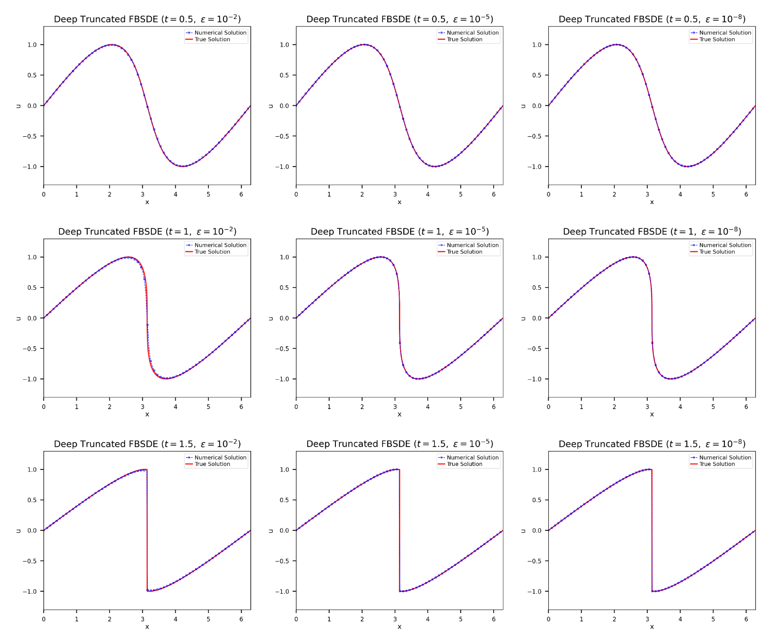
Figure 2. Deep truncated FBSDE method for the one-dimensional Burgers equation. Rows correspond to T=0.5,1.0,1.5, and columns correspond to \varepsilon=10^{-2},10^{-5},10^{-8}. Figure courtesy of the authors.
A heterogeneous 100-dimensional test. We next consider a spatially heterogeneous, 100-dimensional extension of a Burgers-type benchmark from the deep BSDE literature [3].
Its coefficients contain coordinate-dependent linear and oscillatory terms, while the exact solution remains known.
We use a coupled FBSDE formulation in which nonlinear convection is represented through the forward dynamics rather than through an explicit high-dimensional Z-dependent term in the backward equation.
This provides a demanding test of the method under heterogeneous coupling in high dimension.
Figure 3 shows the relative error and the predicted solution value over training, based on 10 independent runs.
With terminal time T=1, the exact value at t=0 and x=(0,\ldots,0) is 0.5.
The final mean relative error is 7.35\times10^{-3}, and the mean predicted value is 0.501514.
Outlook
The deep truncated FBSDE method preserves the coupled stochastic dynamics while reducing the unstable feedback created by parameter-dependent forward paths. The Burgers experiments show its behavior in nearly inviscid and post-shock regimes, while the 100-dimensional example illustrates how the method can approximate selected solution values without constructing a full spatial grid. More broadly, the coupled formulation allows nonlinear transport to be represented through the forward dynamics, avoiding singular generator terms in the corresponding decoupled BSDE. These results suggest that the method provides a scalable framework for both low- and high-dimensional problems, particularly when strong coupling, long-time propagation, or nonlinear transport makes existing BSDE-based solvers challenging to train. Future work will explore broader classes of nonlinear PDEs and coupled stochastic systems.
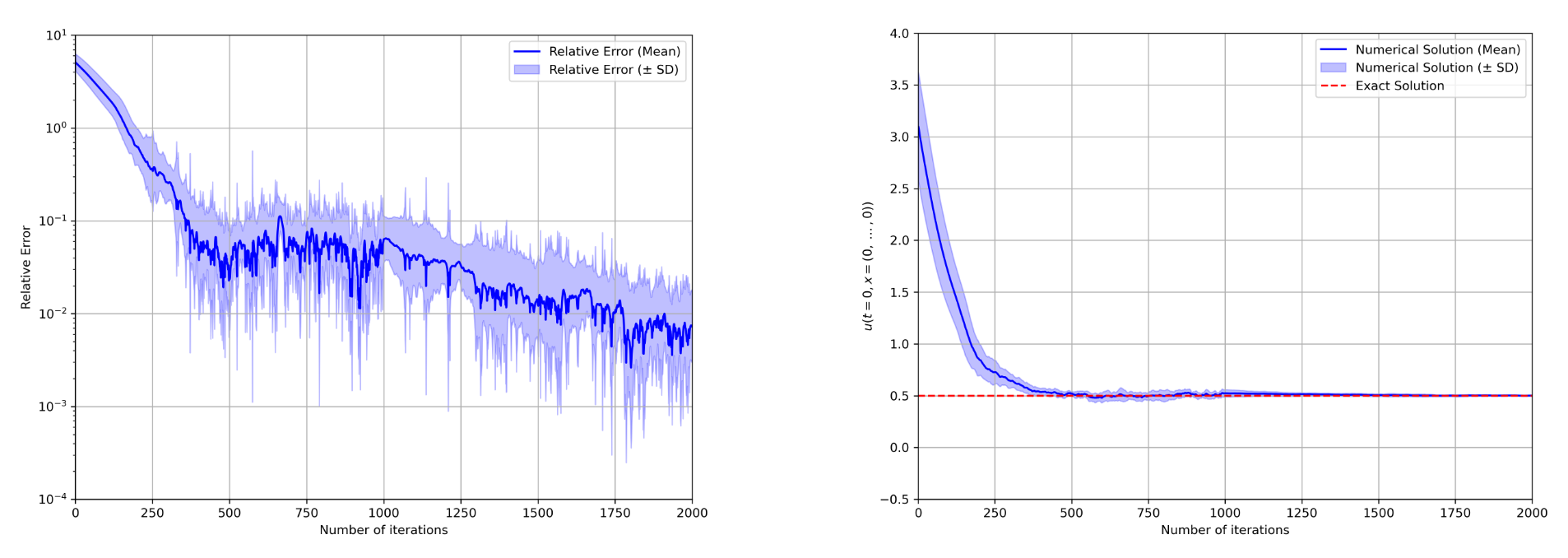
Figure 3: Results for the 100-dimensional spatially heterogeneous Burgers-type equation, based on 10independent runs. Left: relative error. Right: numerical value at t = 0 and x = (0, . . . , 0). Figure courtesy of the authors.
References
[1] Andersson, K., Andersson, A., & Oosterlee, C. W. (2026). The deep multi-FBSDE method: A robust deep learning method for coupled FBSDEs. J. Sci. Comput., 106 (3), Paper No. 77, 23.[2] Cheng, X., Li, Y., Xiong, W., & Zuazua, E. (2026). The deep truncated FBSDE method: A robust solver for high-dimensional PDEs [Unpublished manuscript].
[3] E, W., Han, J., & Jentzen, A. (2017). Deep learning-based numerical methods for highdimensional parabolic partial differential equations and backward stochastic differential equations. Commun. Math. Stat., 5 (4), 349–380.
[4] Han, J., Jentzen, A., & E, W. (2018). Solving high-dimensional partial differential equations using deep learning. Proc. Natl. Acad. Sci. USA, 115 (34), 8505–8510.
[5] Huré, C., Pham, H., & Warin, X. (2020). Deep backward schemes for high-dimensional nonlinear PDEs. Math. Comp., 89 (324), 1547–1579.
[6] Ji, S., Peng, S., Peng, Y., & Zhang, X. (2020). Three algorithms for solving high-dimensional fully coupled FBSDEs through deep learning. IEEE Intelligent Systems, 35 (3), 71–84.
[7] LeVeque, R. J. (1992). Numerical methods for conservation laws (Second). Birkhäuser Verlag, Basel.
[8] Pardoux, E., & Tang, S. (1999). Forward-backward stochastic differential equations and quasilinear parabolic PDEs. Probab. Theory Related Fields, 114 (2), 123–150.
[9] Zhang, W., & Cai, W. (2022). FBSDE based neural network algorithms for high-dimensional quasilinear parabolic PDEs. J. Comput. Phys., 470, Paper No. 111557, 14.
About the Authors
Xinyu Cheng
Young Principal Investigator, Research Institute of Intelligent Complex Systems, Fudan University
Xinyu Cheng received his Ph.D. in mathematics from the University of British Columbia. His research focuses on the theory, modeling, and interdisciplinary applications of space–time dynamical equations in complex systems.
Yunzhang Li
Associate Principal Investigator, Research Institute of Intelligent Complex Systems, Fudan University; Visiting Scientist, Department of Mathematics, Friedrich-Alexander-Universität Erlangen–Nürnberg
Yunzhang Li received his Ph.D. from the School of Mathematical Sciences at Fudan University. His research focuses on high-order numerical algorithms for optimal control problems of stochastic systems.
Weiran Xiong
Ph.D. Student, Research Institute of Intelligent Complex Systems, Fudan University
Weiran Xiong’s research interests include scientific machine learning, stochastic optimal control, and reinforcement learning.
Enrique Zuazua, Chair for Dynamics, Control and Numerics, Friedrich-Alexander-Universität Erlangen–Nürnberg
Enrique Zuazua holds the Chair for Dynamics, Control and Numerics–Alexander von Humboldt Professorship in the Department of Data Science at Friedrich-Alexander-Universität Erlangen– Nürnberg in Germany. He also has part-time appointments at Universidad Autónoma de Madrid and the DeustoCCM at University of Deusto in Spain.