
Authors: Jun Chen, Umberto Biccari, Junmin Wang
Imagine a system that must adapt as conditions change. A robot may encounter a different load, an aircraft may move into a new flight regime, or a digital twin may incorporate fresh measurements. In each case, changing conditions can alter the underlying model and require a new control strategy. With conventional numerical methods, each new problem is generally treated as a fresh calculation, even when it differs only slightly from the previous one. A single calculation may be routine, but repeating it hundreds or thousands of times can become the real computational obstacle.
Neural operators offer a different way to organize this work. Instead of memorizing one answer, they learn how a whole family of problems is connected to its answers. The computational effort is invested upfront, using carefully generated examples to teach the model. Once trained, it can respond quickly whenever new information arrives.
Feedback control makes the value of this approach especially clear, because the quality of an approximation has an immediate practical meaning. A feedback controller continually observes a system and corrects its behavior. It might keep a drone on course, steady a robotic arm, or help a vehicle respond to changing road conditions. To decide how strongly to react, the controller must balance two goals: keeping the system close to its desired behavior and avoiding unnecessary control effort. This balancing act lies at the heart of the linear-quadratic regulator (LQR). Finding the best response requires solving a Riccati equation, which produces the recipe that the controller uses to react to the current state of the system.
For LQR, this general idea becomes a specific task [1]. A Deep Operator Network, or DeepONet [2], combines two kinds of information: how the system changes and the time at which a response is needed. Its output approximates the Riccati solution from which the feedback strategy is built.
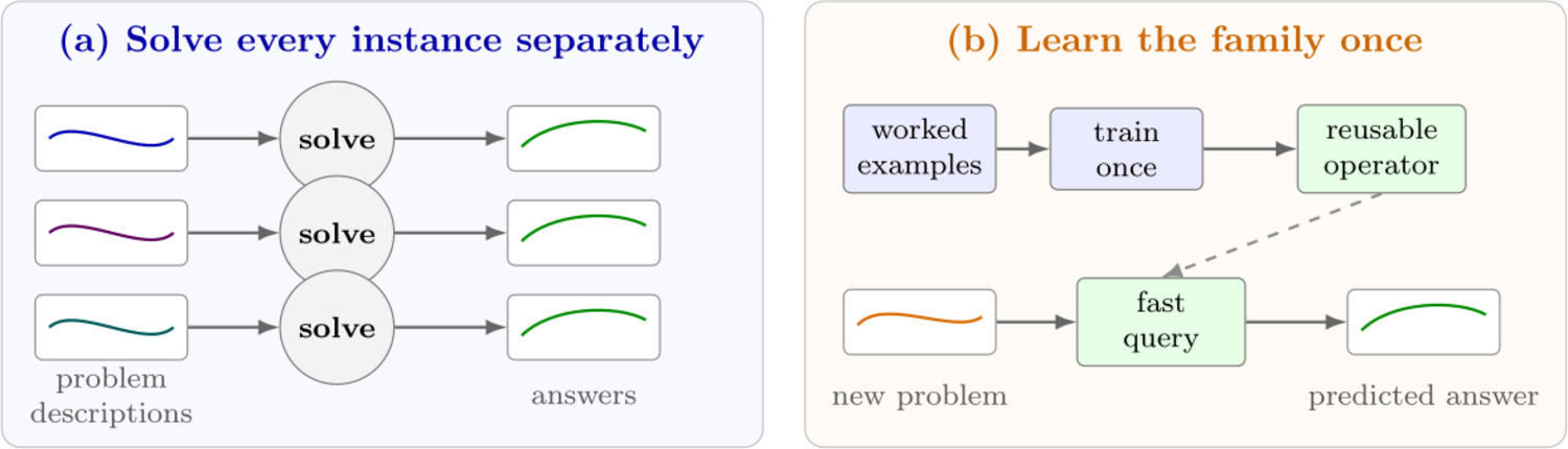
This approach comes with a clear bargain: invest more time at the beginning in exchange for faster answers later. Preparing the examples and training the network can take hours, so the investment only makes sense when many related problems are expected.
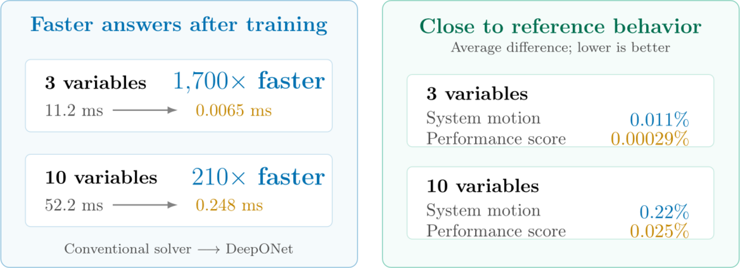
When that condition is met, the payoff can be dramatic. On the same laptop, producing a new solution for a three-variable system took about 11.2 milliseconds with the conventional solver and just 0.0065 milliseconds with DeepONet. For a 10-variable system, the times were 52.2 and 0.248 milliseconds. Put differently, the learned model was roughly 1,700 times faster in the smaller case and 210 times faster in the larger one. A fraction of a millisecond may seem insignificant, but such savings accumulate when a calculation must be repeated again and again.
The more revealing result, however, concerned what happened after the answer left the network and entered the feedback loop. For 10-dimensional models, the predicted Riccati solution differed from the reference by about eight percent. Yet the motion of the controlled system differed by only about 0.22 percent, and its overall performance score by roughly 0.025 percent. The lesson is important: the quality of a learned controller cannot be judged solely by an intermediate mathematical error. What ultimately matters is how the controlled system behaves.
Speed and numerical agreement are not the whole story. A feedback strategy must also prevent small disturbances from growing. Figure 3 turns this question into a visual test: points on the left side of the dashed boundary represent responses that fade over time, while points on the right represent responses that grow. The two panels have nearly the same overall shape, indicating that the learned strategy usually preserves the stabilizing effect of the conventional one.
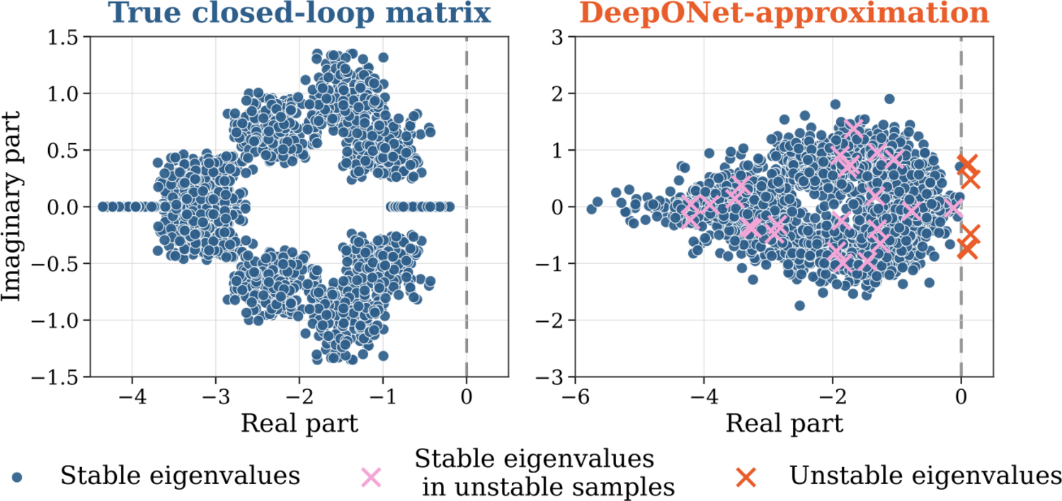
The few orange crosses beyond the boundary are just as informative as the large cluster of successful predictions. They show that the learned strategy is not infallible and that speed must be accompanied by a way to recognize uncertain cases. Here, control theory supplies such a check. The analysis provides a safety margin: when the learned answer is close enough to the reference, the stability of the conventional controller is guaranteed to carry over. Falling outside this margin does not predict failure, but it does flag a case that deserves closer inspection.
Every unstable prediction in the 10-variable test fell outside the conditions covered by this guarantee. In a broader set of three-variable tests, the learned strategy preserved stability in more than 99.99 percent of the stable cases across 10 independent trials. Seen in this light, the rare exceptions are not merely blemishes in an accuracy table; they illustrate how mathematical safeguards can work alongside a learned model.
Another question is whether the approach can grow with the systems it is meant to control. Larger systems contain many more interacting quantities, which makes both training and prediction harder. An initial experiment offered one possible route forward: a model for a four-variable system reused information from a three-variable model. Compared with building the larger model from scratch, this reduced the number of adjustable parameters by about 95 percent and training time by 77 percent, with only a modest loss of accuracy. The result is not a general scaling solution, but it suggests that knowledge learned for one system size may be useful for another.
These experiments were designed to test the idea, not to certify a ready-to-deploy controller. The systems were computer generated and moderate in size, and the test cases resembled the examples used during training. How the model behaves under genuinely unfamiliar conditions remains an open question. Future designs could also build more of the known mathematical structure directly into the network, rather than asking it to recover everything from examples.
LQR is just one example of the broader opportunity. Similar repeated calculations appear in fluid simulation, materials design, weather prediction, medical modeling, and many other areas. The details differ, but the central question remains the same: when a family of related problems must be solved again and again, can earlier calculations be turned into a reusable tool?
The Riccati example offers a qualified yes. The initial training cost must be recovered through repeated use, new problems must remain reasonably close to the training examples, and accuracy must be measured by what matters in the application. Neural operators do not replace conventional solvers or mathematical analysis. Their promise is to combine both into a fast reusable model—and to identify when that model can be trusted.
References
[1] J. Chen, U. Biccari & J. Wang (2026). Learning the Riccati solution operator for time-varying LQR via Deep Operator Networks. arXiv preprint.[2] L. Lu, P. Jin, G. Pang, Z. Zhang & G.E. Karniadakis (2021). Learning nonlinear operators via DeepONet based on the universal approximation theorem of operators. Nature Machine Intelligence, 3(3), 218-229.
|| Go to the CoDeFeL blog main page