
Learning the Riccati solution operator for time-varying LQR via Deep Operator Networks
 Jun Chen
 Umberto Biccari
 Junmin Wang
This post provides an overview of the results in the paper:
J. Chen, U. Biccari & J. Wang (2026). Learning the Riccati solution operator for time-varying LQR via Deep Operator Networks, arXiv preprint arXiv:2604.18507
GitHub Repository
Resources available at our repo at FAU DCN-AvH GitHub
Introduction
We propose a computational framework for replacing the repeated numerical solution of differential Riccati equations in finite-horizon Linear Quadratic Regulator (LQR) problems by a learned operator surrogate. Instead of solving a nonlinear matrix-valued differential equation for each new system instance, we construct offline an approximation of the associated solution operator mapping time-dependent system parameters to the Riccati trajectory.
Consider the finite-horizon Linear Quadratic Regulator (LQR) problem for continuous-time linear time-varying system. The system dynamics are given by
\begin{cases} \dot{x}(t) = A(t)x(t) + B(t)u(t),\quad t\in[0,T], \\ x(0) = x_0, \qquad (1) \end{cases}
where x( \cdot ) \in\Reals^n, u( \cdot ) \in\Reals^m, A( \cdot )\in\Reals^{n\times n} and B( \cdot )\in\Reals^{n\times m}. The LQR controller is designed by minimizing the quadratic cost functional
J(u) = \int_0^T \Big(x(t)^\top Q(t)x(t) + u(t)^\top R(t)u(t) \Big)\, dt + x(T)^\top P_T x(T), \qquad (2)
where Q( \cdot )\in\Reals^{n\times n}, R( \cdot )\in\Reals^{m\times m} are symmetric matrices, with Q positive semi-definite and R postive definite, and P_T\in\Reals^{n\times n}.
It is well known [1] that, under standard stabilizability and detectability assumptions, the optimal control is given in feedback form
u^\ast(t)=-K^\ast(t)x(t), \quad\text{ with } K^\ast(t)=R^{-1}(t)B^\top(t)P^\ast(t),
where P^\ast(t) is the unique symmetric positive definite solution of the Differential Riccati Equation (DRE)
\begin{cases} -\dot{P}(t) = A(t)^\top P(t) + P(t)A(t) - P(t)B(t)R^{-1}(t)B(t)^\top P(t) + Q(t), \; t\in[0,T] \\[2pt] P(T) = P_T. \qquad (3) \end{cases}
Despite its conceptual simplicity, the practical deployment of LQR in modern applications is, however, often hindered by computational challenges. In particular, classical numerical methods, typically very effective for solving a single instance of (3), may become prohibitive in settings where one must evaluate optimal feedback laws for a large number of system configurations. Such situations arise naturally in parametric control, uncertainty quantification, and real-time applications like Model Predictive Control (MPC), where optimal control problems must be solved sequentially in real time for evolving system states and parameters.
To overcome this bottleneck, we propose an Operator Learning (OL) viewpoint to approximate the Riccati solution operator
\mathcal F : \Theta \mapsto P( \cdot ),
where \Theta = (A( \cdot ), B( \cdot ), Q( \cdot ), R( \cdot ), P_T) denotes the collection of system parameters, which associates to each parameter instance the corresponding solution of the DRE (3).
OL approximation of the Riccati operator
We first formulate the exact mapping from system parameters to the solution of the DRE. To this end, we introduce the following notation:
Let \mathbb{S}^n denote the n\times n real symmetric matrices, with \mathbb{S}^n_+ and \mathbb{S}^n_{++} the positive semidefinite and positive definite subsets. For A,B\in\mathbb{S}^n, A\succeq B means A-B\in\mathbb{S}^n_+, and A\succ B means A-B\in\mathbb{S}^n_{++}. Define
\Sigma_{++}^m \coloneqq \left\{ R:[0,T]\to\mathbb{S}^m_{++} \; \big| \; \exists\rho>0,\; R(t)\succeq\rho I_m\ \forall t\in[0,T] \right\},
with I_m the m\times m identity. For a matrix A, \|A\|_F is the Frobenius norm; for a vector x, \|x\|_2 is the Euclidean norm.
Let \Theta = (A( \cdot ), B( \cdot ), Q( \cdot ), R( \cdot ), P_T), and define the admissible input space
\mathcal{X} = \left\{\Theta \;\text{ s. t. }\; \begin{array}{l} \begin{array}{lll} A \in C([0,T]; \mathbb{R}^{n\times n}) & B \in C([0,T]; \mathbb{R}^{n\times m}) \\ Q \in C([0,T]; \mathbb{S}^n_+) & R \in C([0,T]; \Sigma_{++}^m) & P_T \in \mathbb{S}^n_{++} \end{array} \\ \; (A(t),B(t)) \text{ is uniformly stabilizable} \\ \; (A(t),Q(t)^{1/2}) \text{ is uniformly detectable} \end{array}\right\}. \qquad (4)
For all \Theta\in\mathcal X, the Riccati equation (3) admits a unique solution P\in C([0,T];\mathbb S_{++}^n) [5,6].
Accordingly, we define the output space
\mathcal Y \coloneqq \Big\{P \in C([0,T];\mathbb S_{++}^n) \;\big|\; P \text{ solves } (3) \text{ for some } \Theta\in\mathcal X\Big\}. \qquad (5)
This choice of spaces allows us to view the Riccati map as an operator
\mathcal F : \mathcal X \mapsto \mathcal Y, \quad \mathcal F(\Theta)=P( \cdot ). \qquad (6)
Operator Learning formulation: the DeepONet architecture
To learn the mapping \mathcal F, we employ a DeepONet for learning mappings between function spaces. The architecture comprises a branch network and a trunk network. The branch network encodes the system parameters \Theta into coefficients \beta_k(\Theta), while the trunk network takes time t and outputs basis functions \tau_k(t). The predicted solution is then
\mathcal G(\Theta)( \cdot ) = \sum_{k=1}^p \beta_k(\Theta)\tau_k( \cdot ) \sim P( \cdot ).
The mapping \mathcal F is well-defined and locally Lipschitz in the parameters [2,3]. Hence, by [4, Theorem 1], for any \varepsilon>0 there exists a DeepONet \mathcal G such that for all \Theta and t\in[0,T],
\big\|\mathcal F(\Theta)(t)-\mathcal G(\Theta)(t)\big\|\lt \varepsilon.
Error propagation and stability analysis of the learned controller
Given an approximate solution \hat P produced by the DeepONet, we now analyze how the approximation error affects the closed-loop performance.
Consider system (1) with quadratic cost (2). For \Theta=(A,B,Q,R,P_T)\in\mathcal X, with \mathcal X as in (4), let P^\ast\in C([0,T];\mathbb S_{++}^n) be the unique solution of the DRE (3). Define:
K^*(t) = R^{-1}(t)B^\top(t)P^*(t), \quad \hat K(t) = R^{-1}(t)B^\top(t)\hat P(t) \quad \text{optimal feedback gain} \qquad (7a)
x^*(t), \quad \hat x(t) \quad \text{optimal state} \qquad (7b)
u^*(t) = -K^*(t)x^*(t), \quad \hat u(t) = -\hat K(t)\hat x(t) \quad \text{optimal control} \qquad (7c)
Let \mathcal{F} and \widehat{\mathcal{F}} denote the exact and learned Riccati operators. The approximation error propagates through the feedback loop as
\hat{\mathcal{F}} \sim \mathcal{F} \;\longrightarrow\; \hat K \sim K^\ast \;\longrightarrow\; \hat x \sim x^\ast \;\longrightarrow\; J(\hat u) \sim J(u^\ast).
The following theorem quantifies the propagation of the operator approximation error through the feedback law.
Theorem 1
Given T>0 and \Theta=(A,B,Q,R,P_T)\in\mathcal X, with \mathcal X as in (4), let P^\ast\in C([0,T];\mathbb S_{++}^n) be the unique solution of the DRE (3). Let \hat P be an approximate solution of (3) obtained by DeepONet, and define the error E(t)\coloneqq \hat P(t) - P^\ast(t). Assume there exists \varepsilon>0 such that
\sup_{t\in[0,T]} \|E(t)\| \lt \varepsilon. \qquad (8)
Then, for any initial datum x_0\in\Reals^n, we have the following
1. Finite–horizon performance error. There exist constants C_1, C_2, C_3, C_4 > 0, depending on \Theta and T, such that the optimal states and controls given by (7b) and (7c) satisfy
\sup_{t\in[0,T]} \|\hat x(t) - x^\ast(t)\|_2 \leq C_1 \|x_0\|_2 \Big(e^{C_2\varepsilon T}-1\Big), \qquad (9)
J(\hat u) - J(u^\ast) \leq C_3\|x_0\|^2_2\varepsilon^2 Te^{C_4\varepsilon T}.
2. Stability of the learned closed–loop system. There exists \varepsilon^\ast=\varepsilon^\ast(\Theta,T)>0 such that if \varepsilon \lt \varepsilon^\ast the approximate optimal state \hat x(t) is uniformly stable on [0,T]. More precisely, there exist constants M(\Theta,T),\mu(\Theta,T) > 0 such that
\|\hat x(t)\|_2 \leq M e^{-\mu t}\|x_0\|_2, \quad \text{for all } t \in [0,T]. \qquad (10)
Simulation
We demonstrate the effectiveness of the DeepONet approach for learning the Riccati operator.
Data Generation
To obtain a representative dataset, system matrices are generated via a truncated trigonometric expansion:
\begin{array}{l} \displaystyle A(t) = A_0 + \sum_{i=1}^{r_{\text{base}}} \Big(C_{1i} \phi_i(t) + C_{2i} \psi_i(t)\Big), \\ \displaystyle B(t) = B_0 + \sum_{i=1}^{r_{\text{base}}} \Big(D_{1i} \phi_i(t)+ D_{2i} \psi_i(t)\Big), \\ \displaystyle Q(t) = M^\top(t) M(t) \quad\text{ with }\quad M(t) = M_0 + \sum_{i=1}^{r_{\text{base}}} \Big(E_{1i} \phi_i(t)+ E_{2i} \psi_i(t)\Big), \qquad (11) \end{array}
with basis functions \phi_i(t)=\cos(i\pi t), \psi_i(t)=\sin(i\pi t).
All coefficients A_0, B_0, M_0, C_{ki}, D_{ki}, E_{ki} with k=1,2 and i= 1,\dots, r_{\text{base}} are sampled from \mathcal{N}(0, 0.05^2). r_{\text{base}}=2.
The control weighting matrix is constant: R(t)=I_m, and the terminal cost is P_T=I_n.
For each sampled instance, we numerically solve the DRE (3) backward using fourth-order Runge-Kutta (RK4).
Only trajectories satisfying uniform stabilizability of (A(t),B(t)) and detectability of (A(t),Q(t)^{1/2}) at all discrete time steps are retained.
For the 3‑dimensional case we obtain 1000 valid trajectories; for the 10‑dimensional case we obtain 3000.
Error Metrics
Let K denotes the number of test trajectories. For each trajectory indexed by k=1,\dots,K, P^{(k)}(t), x^{(k)}(t), and J^{(k)} represent the ground-truth Riccati solution, state trajectory, and cost functional, respectively, while \hat{P}^{(k)}(t), \hat{x}^{(k)}(t), and \hat{J}^{(k)} denote their corresponding DeepONets predictions. We define the following average errors:
\begin{array}{ll} \text{Riccati solution errors} \\ \displaystyle e_P = \frac 1K \sum_{k=1}^K \left(\int_0^T \| P^{(k)}(t) - \hat{P}^{(k)}(t) \|_F^2 \, dt \right)^{\frac 12} & \quad \text{absolute error} \\[15pt] \displaystyle e_P^r = \frac 1K \sum_{k=1}^K \left( \int_0^T \| P^{(k)}(t) \|_F^2 \, dt \right)^{-\frac 12} \left( \int_0^T \| P^{(k)}(t) - \hat{P}^{(k)}(t) \|_F^2 \, dt \right)^{\frac 12} & \quad \text{relative error} \\[25pt] \text{State errors} \\ \displaystyle e_x = \frac 1K \sum_{k=1}^K \left( \int_0^T \| x^{(k)}(t) - \hat{x}^{(k)}(t) \|_2^2 \, dt \right)^{\frac 12} & \quad \text{absolute error} \\[15pt] \displaystyle e_x^r = \frac 1K \sum_{k=1}^K \left( \int_0^T \| x^{(k)}(t) \|_2^2 \, dt \right)^{-\frac 12}\left( \int_0^T \| x^{(k)}(t) - \hat{x}^{(k)}(t) \|_2^2 \, dt \right)^{\frac 12} & \quad \text{relative error} \\[25pt] \text{Cost functional errors} \\ \displaystyle e_J = \frac 1K \sum_{k=1}^K \left| J^{(k)} - \hat{J}^{(k)} \right| & \quad \text{absolute error} \\[15pt] \displaystyle e_J^r = \frac 1K \sum_{k=1}^K \frac{\left| J^{(k)} - \hat{J}^{(k)} \right|}{\left| J^{(k)} \right|} & \quad \text{relative error} \end{array}
Numerical Results
We generate K=100 test trajectories from parameters not seen during training. Table 1 reports the errors for dimensions n=3 and n=10. The DeepONet predictions are accurate, with errors remaining small even in the 10‑dimensional case, confirming good generalization.
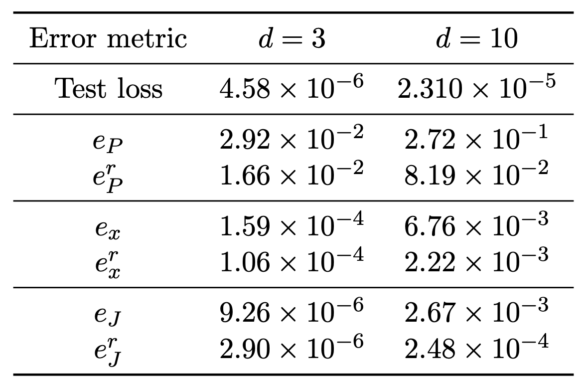
Table 1. Average absolute and relative errors for P(t), state x(t), and cost J in different dimensions.
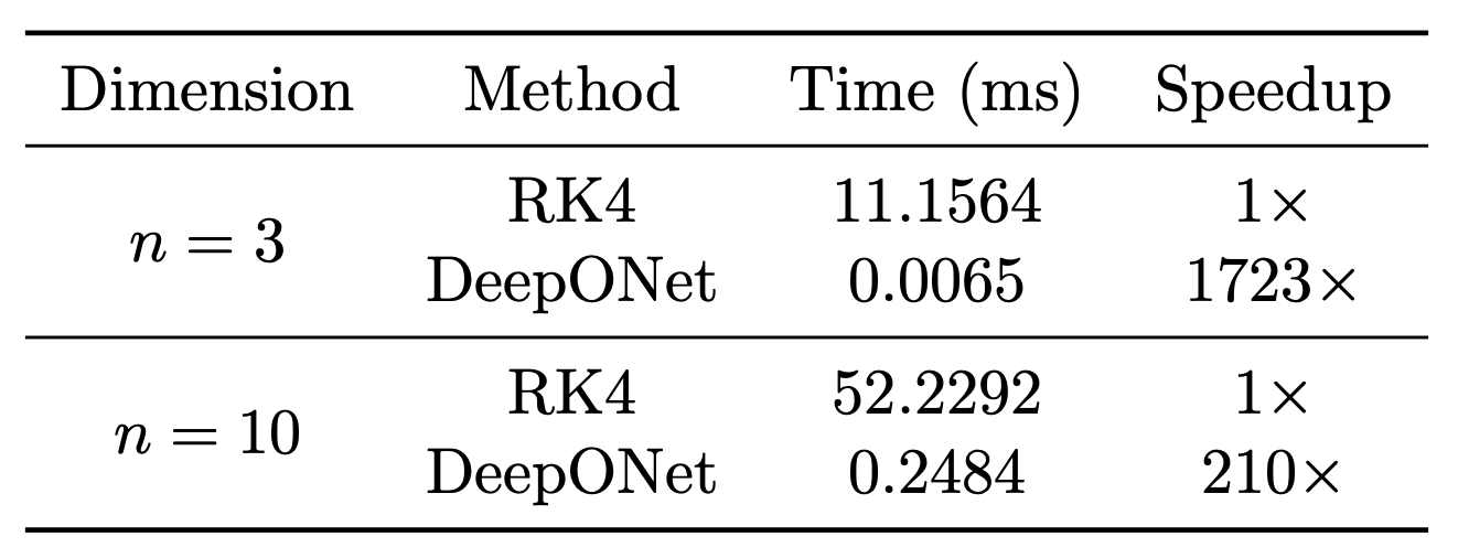
Table 2. Comparison of computational efficiency for solving DRE using RK4 and DeepONet
Once trained, the learned operator evaluates up to several hundred times faster than solving the DRE numerically (Table 2).
Figure 1 compares the true and predicted state trajectories and control inputs for a representative 3‑dimensional test system, the excellent agreement demonstrates the effectiveness of the DeepONet-based controller.
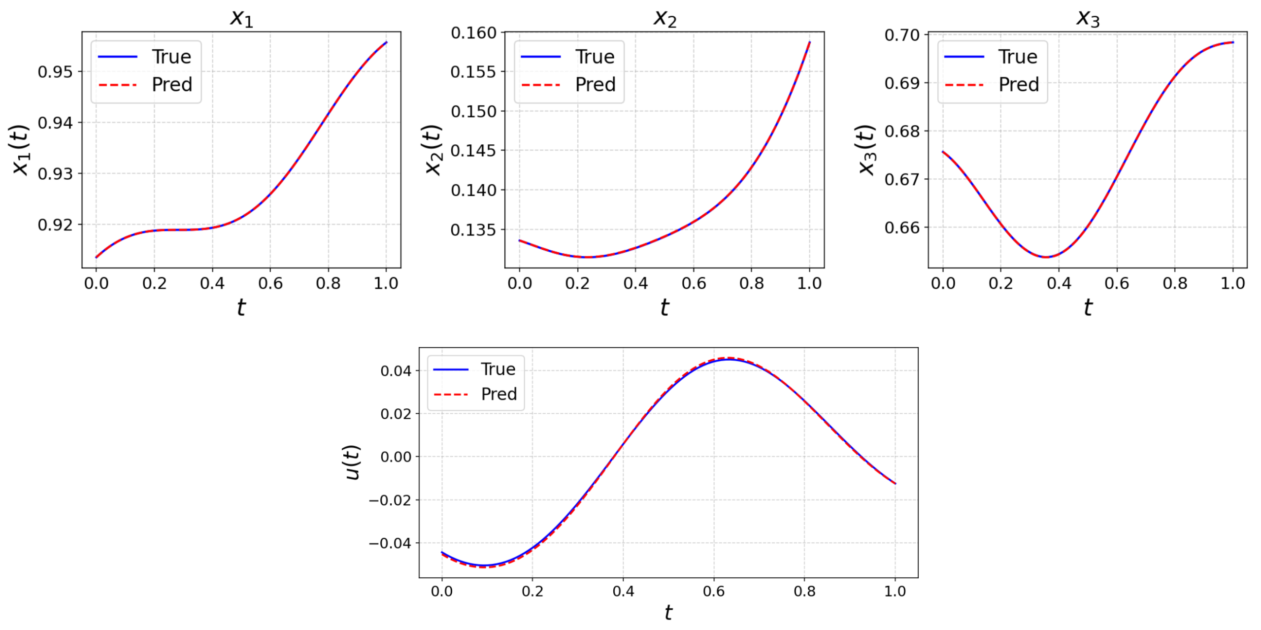
Figure 1. Comparison of predicted and true trajectories (top) and predicted and true controls (bottom) for a 3-d test system.
Conclusion & Outlook
We introduced an operator learning framework for the finite-horizon LQR problem, using DeepONet to approximate the Riccati solution map. Theoretically, we derived explicit bounds linking the operator approximation error to suboptimality and proved that closed-loop exponential stability is preserved when the error is sufficiently small. Numerically, our method achieves up to three orders of magnitude speedup over classical solvers while maintaining high accuracy across dimensions.
The results open several avenues for future investigation:
• Generalization: Derive a priori sample complexity estimates to guarantee a desired control performance, and understand how these bounds scale with system dimension, time horizon, and coefficient regularity.
• Structure preservation: Design neural operator architectures that inherently enforce symmetry and positive definiteness of the learned Riccati solution, ensuring stability without requiring post-processing or threshold conditions.
• Nonlinear and constrained problems: Extend the framework to Hamilton-Jacobi-Bellman equations for nonlinear control, and to model predictive control with state and input constraints, addressing increased operator complexity and regularity challenges.
[2] H. Abou-Kandil, G. Freiling, V. Ionescu, G. Jank (2012) Matrix Riccati equations in control and systems theory, Birkhäuser
[3] S. Bittanti, A. Laub, J. Willems (1991) The Riccati equation, Springer-Verlag
[4] L. Lu, P. Jin, G. Pang, Z. Zhang, G.E. Karniadakis (2021) Learning nonlinear operators via DeepONet based on the universal approximation theorem of operators, Nature Mach. Intell. Vol. 3 No. 3, pp. 218–229.
[5] E.D. Sontag (2013) Mathematical control theory: deterministic finite dimensional systems, Vol. 6, Springer Science & Business Media
[6] B.D. Anderson, J. B. Moore (2007) Optimal control: linear quadratic methods, Courier Corporation
|| Go to the CoDeFeL blog main page