
Authors: Ziqian Li, Kang Liu, Yongcun Song, Hangrui Yue, and Enrique Zuazua
Learning a family of PDE solutions by making time evolution part of the model.
A simulation rarely ends with a single answer. An engineer changes a material, a scientist explores an uncertain forcing, or a designer compares possible interventions. Each change asks the same mathematical model a new question. For systems governed by partial differential equations (PDEs), answering may require another computation of how an entire spatial field evolves.
Consider diffusion and reaction: a quantity spreads through a medium while local interactions change its concentration. Different material properties and source distributions produce different histories. A conventional solver can calculate each history accurately. When thousands of histories are needed for design, uncertainty assessment, or control, the accumulated cost becomes consequential.
This repeated-query setting motivates a complementary computational strategy: use carefully generated simulations to learn a reusable model for a family of problems. The central question is how to make that model reflect both the relationships between different inputs and the physical evolution within each simulation.
Operator learning addresses the first part of this question. An operator is a map between functions. A spatially varying source is a function; the resulting concentration field, changing across space and time, is another. The solution operator connects them. It can also take several input functions, such as a material coefficient together with a source, or an initial fluid state together with an external forcing.
Training examples therefore represent different physical conditions and their corresponding solutions. After training, the model is asked to predict solutions for new conditions within the problem family. The learning effort is invested in a relationship that can be used repeatedly. Our work develops a framework called the neural ordinary differential equation operator network, or NODE-ONet. Its organizing principle is that time-dependent solution operators should be represented through an evolving state. Here, the state evolves in the physical time of the PDE. This brings the dynamical structure of PDEs into the design of an operator-learning model.
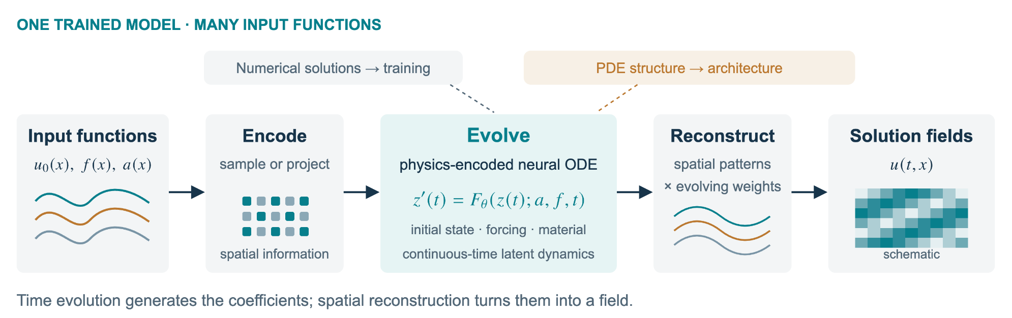
Figure 1. From functions to evolving fields. NODE-ONet encodes spatial inputs, advances a latent state, and reconstructs the solution. The ODE uses encoded coefficient and source inputs; initial data set its starting state. Numerical solutions supply training examples; the PDE guides the neural dynamics. The output field is schematic.
Learning how solutions evolve
Classical numerical methods often handle space and time in separate stages. A spatial discretization replaces a field by finitely many quantities. A time integrator advances those quantities according to an ordinary differential equation. NODE-ONet adopts a related division of work, with trainable components.
First, an encoder converts the input functions into finitedimensional representations. A neural ordinary differential equation then describes how a compact internal, or latent, state evolves continuously in time. A numerical ODE solver advances this state. Finally, a spatial decoder reconstructs the physical field from that state. Initial data determine the starting state, while coefficients and sources influence its subsequent evolution.
The evolving latent variables act as weights for spatial patterns, which can be learned or supplied by a classical basis. The paper also explores reusing a learned spatial decoder for a related equation while retraining its dynamics.
The equation provides a further guide: it suggests how the latent state should evolve. We incorporate selected relationships directly into the neural dynamics.
In the diffusion-reaction example, external forcing enters additively. The diffusion coefficient couples multiplicatively with the evolving state. The network builds these distinct interactions into its evolution model. In the two-dimensional Navier–Stokes example, the dynamics include quadratic interactions inspired by fluid advection. Explicit, low-degree dependence on time keeps the model compact.
Encoding physics in this way means building equation structure into the architecture. Parameters are fitted to numerical PDE solutions, combining information from the equations and simulations.
To understand where approximation errors arise, the paper also analyzes a general encoder-decoder architecture. The analysis separates the effects of input representation, intermediate approximation, and output reconstruction. The experiments test prediction beyond the training time interval; the analysis does not guarantee accurate longtime prediction.
What the experiments show
Two nonlinear diffusion-reaction benchmarks illustrate what the dynamical design can achieve.
With both the diffusion coefficient and source varying, NODE-ONet achieves a relative test error of 1.032%, compared with 2.072% for MIONet, a network for multiple input functions. Both use 1,000 training input pairs. NODE-ONet has 28,550 trainable parameters, versus 161,600, approximately 82% fewer. Its temporal training resolution is 10 steps, versus 100 for MIONet. This experiment demonstrates useful accuracy with a smaller model and a coarser training grid.
The second test examines prediction beyond the training times. For the source-to-solution operator, both models train on 500 input functions over [0, 1] and are evaluated over [0, 2]. Relative errors across that entire evaluation interval are 0.7113% for NODE-ONet and 23.60% for the compared DeepONet, a widely used operator-learning architecture. Figure 2 marks both intervals.
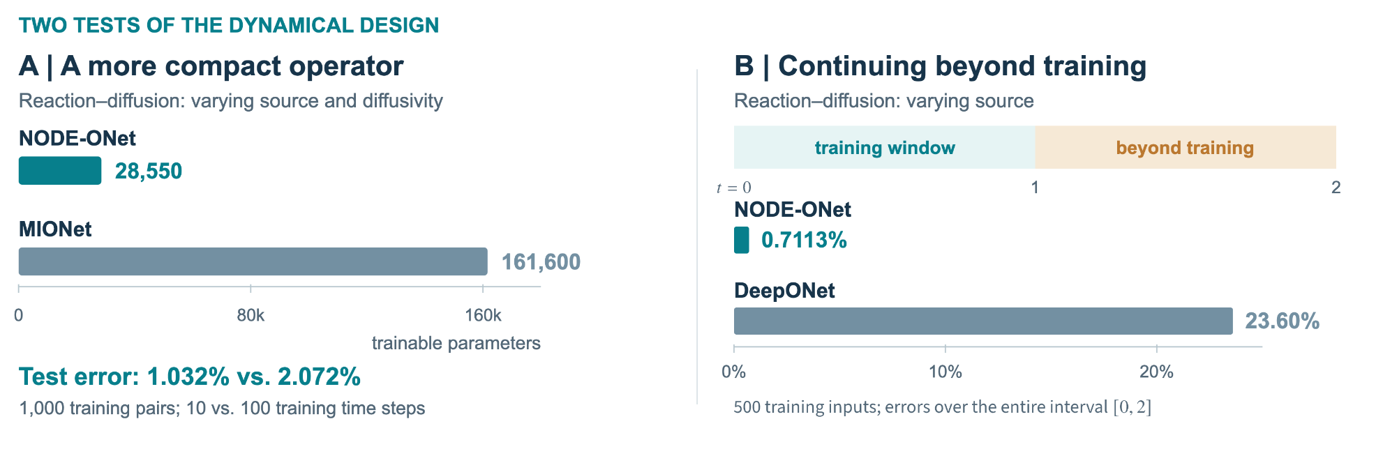
Figure 2. Two reaction–diffusion benchmarks. A: both source and diffusivity vary (Table 5). B: the source varies, with training on [0, 1] and evaluation on the entire interval [0, 2] (Table 6). These are different tests; bars use linear scales. Errors are relative ^2 errors.
The fluid experiments broaden the demonstration. Models learn operators with varying initial vorticity, varying forcing, or both. Training covers times from 0 to 10, and evaluation continues to 20. These tests show how the same architectural principle accommodates different inputs and nonlinear flow evolution; they do not include a comparison with another fluid-learning method.
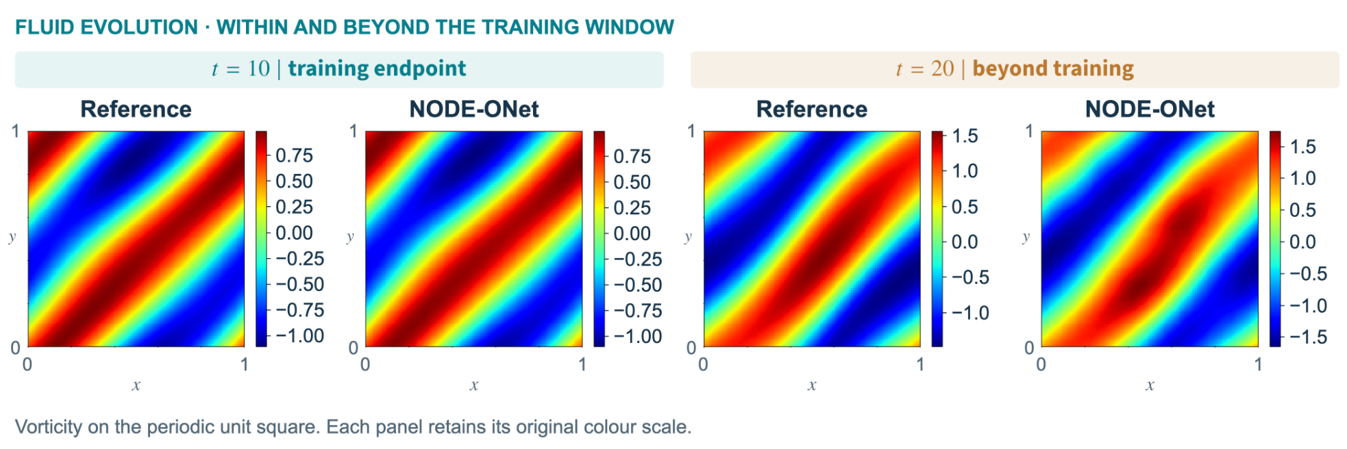
Figure 3. A learned operator for fluid evolution. Vorticity in a two-dimensional Navier–Stokes test, with a new initial condition: numerical reference and NODE-ONet at the training endpoint = 10 and beyond it at = 20. Each panel retains its own original color scale. Adapted from Figure 15 of the paper; this example illustrates one input.
These results support a particular way of designing scientific learning systems: give the learned model a computational structure that reflects the process it represents. Operator learning supplies reuse across input conditions; neural dynamics supply temporal evolution; physics encoding guides the interactions between them.
Practical questions remain. Training requires reference simulations and optimization. Accuracy depends on the represented problem family, the available data, and the chosen architecture. Longer-time prediction needs further analysis and validation, especially where errors grow rapidly. Choosing an effective latent dimension and the appropriate physical structure remains part of the modeling task.
For control, the prospect is valuable: reusable models could help evaluate many candidate actions before selecting an intervention. This connects the work with the ERC project CoDeFeL and its dialogue between control and deep learning. The present results provide a basis for that direction, with scientific computing serving as both the source of training data and the guide to model design.
Research code: NODE-ONet.
Supported in part by the ERC Advanced Grant CoDeFeL: Control for Deep and Federated Learning (ERC-2022-ADG-101096251).
References
[1] Z. Li, K. Liu, Y. Song, H. Yue, and E. Zuazua. Deep neural ODE operator networks for PDEs. Math. Models Methods Appl. Sci. 36(8) (2026), pp. 1739–1782. DOI: 10.1142/S0218202526420054.[2] L. Lu, P. Jin, G. Pang, Z. Zhang, and G. E. Karniadakis. Learning nonlinear operators via DeepONet based on the universal approximation theorem of operators. Nat. Mach. Intell. 3(3) (2021), pp. 218–229. DOI: 10.1038/s42256-021-00302-5.
[3] P. Jin, S. Meng, and L. Lu. MIONet: learning multiple-input operators via tensor product. SIAM J. Sci. Comput. 44(6) (2022), pp. A3490–A3514. DOI: 10.1137/22M1477751.