
Authors: Umberto Biccari, Jun Chen, Roberto Morales, Enrique Zuazua
Imagine trying to infer the properties of a material or a fluid when no single model can see all the measurements. One dataset may describe one part of the system, while another covers a different region or time interval. Gathering everything in one place may be inconvenient, expensive, or impossible.
Bi-Objective Hybrid-Cooperative Learning, or Bi-HYCO, explores another possibility. It keeps a physics-based numerical model and a flexible data-driven model as separate partners. Each works with its own observations, but they regularly compare what they predict for the same physical system [1].
The key idea is simple: the models do not need to exchange raw measurements in order to communicate. They can instead compare their predicted states at agreed locations. If their predictions disagree, both receive information that can guide the next update.
Two complementary views of one system
The first partner is a numerical solver built from the governing physical equations. It offers structure and interpretability: changes in a material coefficient, viscosity, or forcing parameter lead to a corresponding physical state. The second partner is a flexible model, represented by a neural network in the reported experiments.
It describes the same state in a different way and can adapt to information that may be difficult for the numerical model to access directly. Here “synthetic” describes this alternative representation; it does not mean that its observations are artificial.
Each partner remains responsible for fitting its own data. This separation follows the broader HYCO philosophy of combining equation-based and flexible representations without forcing one to replace the other [2]. Figure 1 shows the communication pattern.
Cooperation without extra measurements
The shared comparison locations are not additional sensors. No measured value is attached to them. They are simply places where both models can make a prediction. A model that has learned something useful from its own dataset can therefore influence its partner through agreement or disagreement at these locations.
This is more than averaging two answers after training. The comparison takes place during the
learning process, so it changes how both partners update their parameters. At the same time,
agreement is not proof that either model is correct. The original observations remain the source
of evidence; interaction is a way to transfer information between representations.
Balancing local accuracy and cooperation
Bi-HYCO has two goals. Each model should explain its own observations, and the two models should remain reasonably consistent with one another. These goals can compete. A very close fit to one local dataset may pull a model away from its partner, while very strong agreement may reduce its ability to represent local details.
The method handles this tension by assigning adjustable importance to the different goals.
Changing these priorities selects a different compromise. In multi-objective language, a good compromise is one where improving one goal would necessarily worsen another. Figure 2 presents this idea and the alternating update process used to search for such a solution.
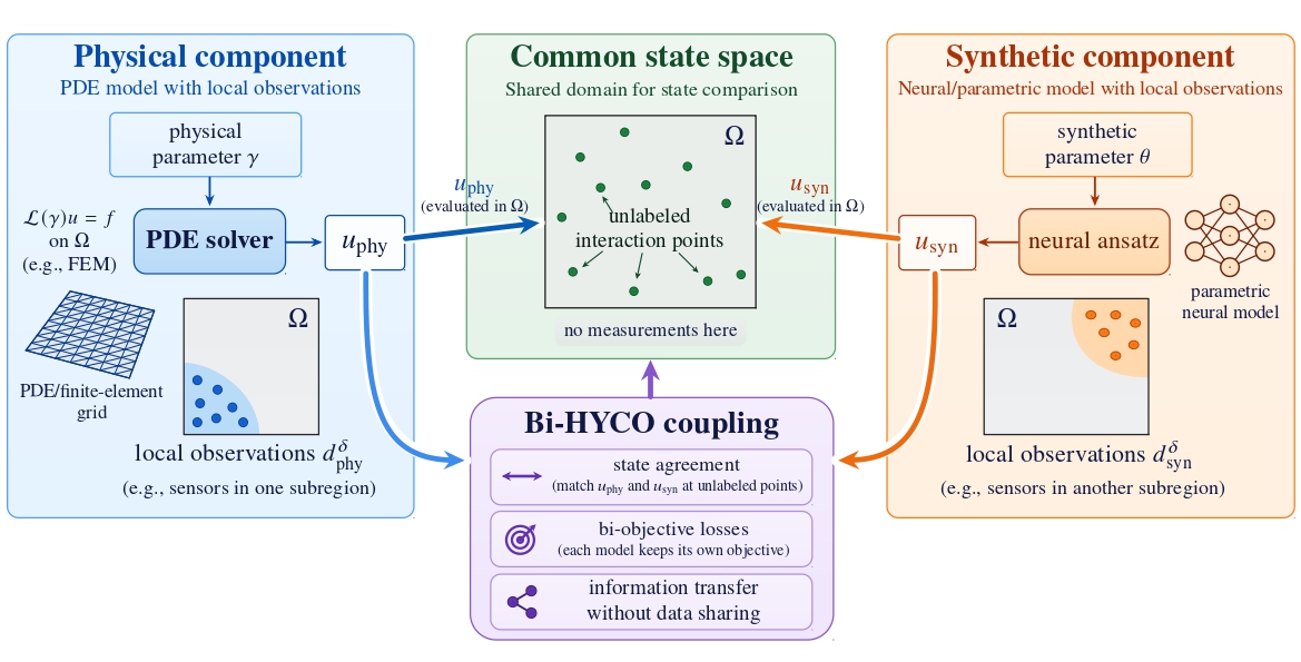
Figure 1: The Bi-HYCO communication mechanism. The physical and synthetic models keep their own
observations but compare predictions at shared locations where no measurements are supplied. This is a
conceptual diagram, not a reconstruction plot. Adapted from Sections 2.1–2.5 of [1].
What the analysis tells us
The paper also studies whether the alternating updates settle down. In a simplified setting with shared observations and fixed comparison points, the answer is yes under a collection of regularity and step-size assumptions: the successive changes become smaller and the full sequence approaches a stable configuration [1, Theorem 3.4].
This result is useful but deliberately limited. It does not guarantee recovery of the true physical parameters, the best possible solution, or convergence of every distributed implementation.
The experiments therefore test a separate practical question: does state interaction add useful information beyond ordinary aggregation of local updates?
Test case 1: a material with an inclusion
The first experiment considers an irregular material containing an inner inclusion. The interface is known, while the material properties on its two sides must be estimated. One local unit observes the state inside the inclusion and another observes the surrounding region. The reconstruction is performed on a different numerical grid from the one used to generate the data, making the test less dependent on a single discretization [1, Section 4].
Bi-HYCO recovers the two material coefficients accurately across the tested noise levels. Removing state interaction produces a modest loss of accuracy in this example, because aggregation alone already performs reasonably well. The detailed field comparison in Figure 3 shows where the methods agree and where small local differences remain.
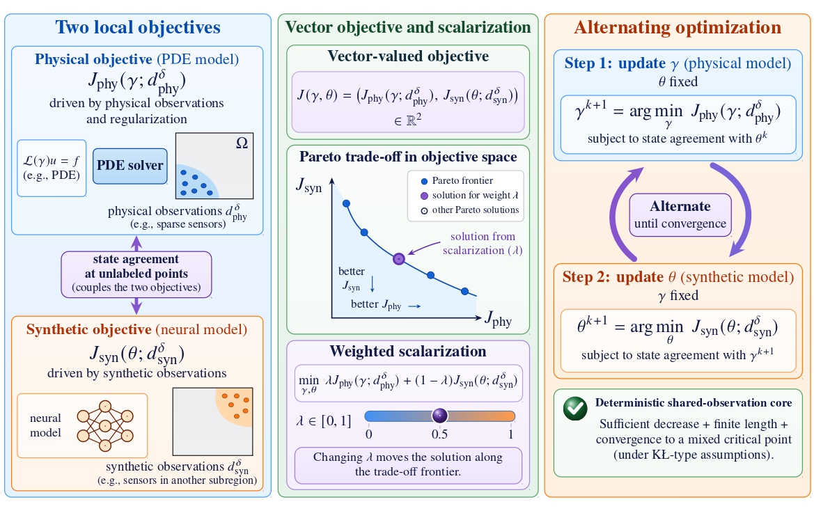
Figure 2: Bi-HYCO balances two local objectives while encouraging agreement between the predicted states. The weights select a point along a range of possible compromises, and the physical and synthetic components are updated in turn. Diagram based on Section 2.3 and Theorem 3.4 of [1].
Test case 2: an evolving flow
The second experiment studies flow around an inner obstacle. The unknown quantities are the fluid viscosity and the strength of the external forcing. Measurements are divided among alternating sectors of the annular domain, so neither local unit sees the whole flow [1, Section 5.1].
Here cooperation has a much larger effect. With the strongest tested noise, the overall parameter error is about 16% with full Bi-HYCO and about 92% when state interaction is removed, while the local optimization and coordinator aggregation remain in place [1, Table 11]. This does not establish a universal advantage, but it shows that interaction can be especially valuable in a nonlinear, time-dependent problem.
Figure 4 compares the final-time spatial patterns produced by the different approaches. The three-dimensional surfaces provide an overall view, while the two-dimensional maps and close-ups make discrepancies near the inner boundary easier to see.
How to read the comparisons
No single method wins every comparison. In the noise-free material experiment, Bi-HYCO reports the smallest parameter and solver-based state errors, but it also takes longer than the PINN and XPINN implementations. In the noise-free flow experiment, XPINN reports the smallest combined parameter error, while Bi-HYCO performs best on the forcing parameter and on the global state reconstructed by the numerical solver [1, Tables 4 and 7].
These results should therefore be read as a collection of trade-offs, not as a universal ranking.
Accuracy, computing time, the chosen representation, and the quantity being measured all affect the comparison. The experiments are fixed realizations rather than repeated statistical trials.
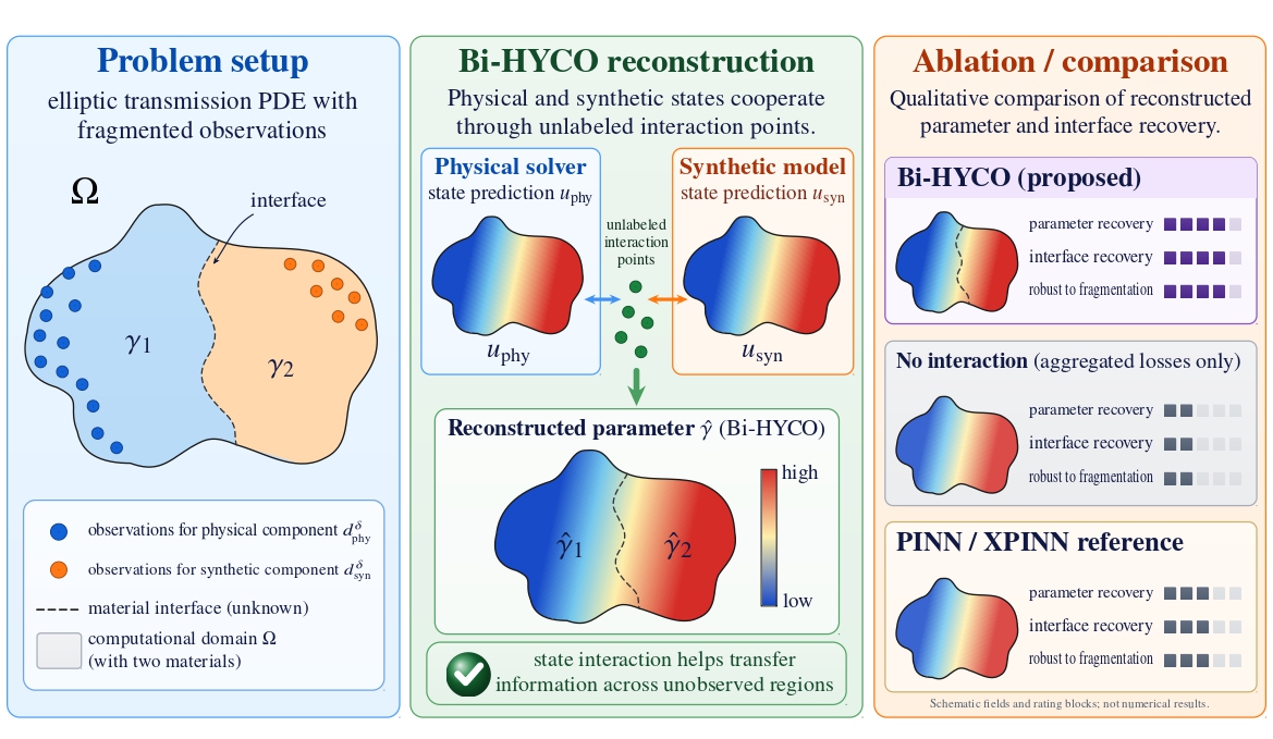
Figure 3: Noise-free elliptic comparison. The columns show the reference field, the physical and synthetic Bi-HYCO reconstructions, a PINN reconstruction, and an XPINN reconstruction. The rows compare the solution, a magnified solution region, the spatial gradient, a magnified gradient region, and reconstruction error. The plots reveal local differences that a single summary number can hide.
The broader message
Bi-HYCO offers a practical form of cooperation for situations in which observations are fragmented.
The models preserve their separate data and distinct strengths, yet exchange information through predictions of the same physical state. The experiments suggest that this interaction can add value beyond simply averaging local parameter updates, particularly when the underlying dynamics are nonlinear.
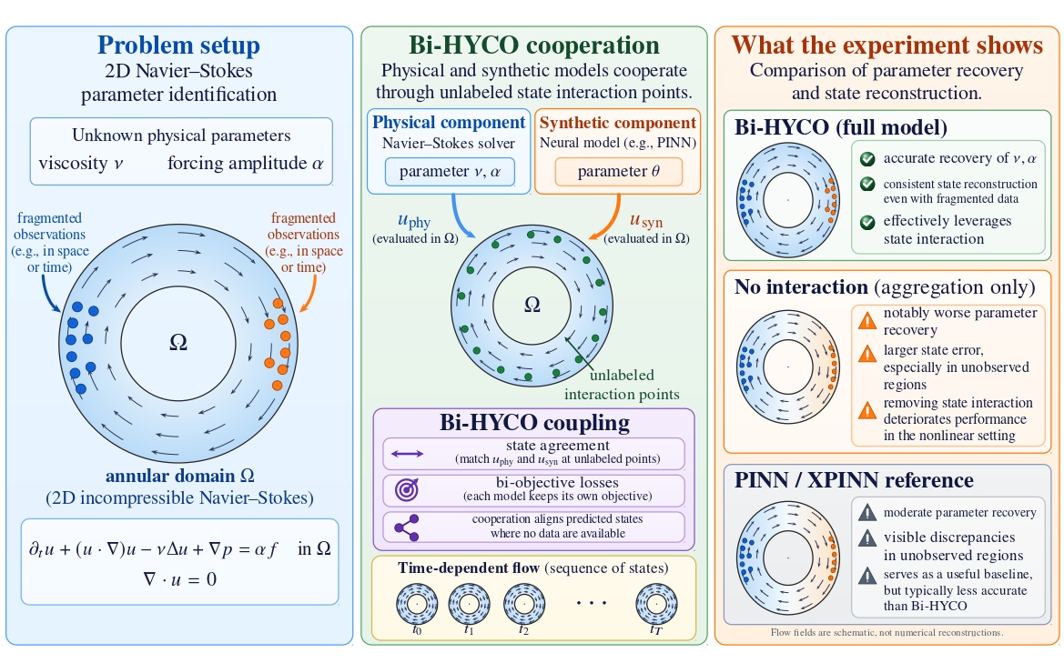
Figure 4: Final-time Navier–Stokes comparison. Columns show the reference gradient field, the physical
and synthetic Bi-HYCO reconstructions, PINN, and XPINN. The top row uses three-dimensional surfaces;
the middle row shows the same patterns from above; and the bottom row enlarges the region near the inner
boundary. These are qualitative field comparisons, while the paper’s tables report the parameter and state
errors.
Important questions remain: how should comparison points be chosen, when does agreement genuinely improve parameter identification, and how well does the approach scale to larger systems?
Those questions define the next stage of the research rather than conclusions already established
by the current experiments [1, Section 6].
References
[1] U. Biccari, J. Chen, R. Morales, and E. Zuazua, Bi-HYCO: Bi-Objective Cooperative Learning for PDE Parameter Identification under Fragmented Observations, arXiv:2609.06511v1, 2026. https://arxiv.org/abs/2609.06511v1.[2] L. Liverani and E. Zuazua, HYCO: A Formalism for Hybrid-Cooperative PDE Modelling, arXiv:2602.23859, 2026. https://arxiv.org/abs/2602.23859.
[3] H. Attouch, J. Bolte, and B. F. Svaiter, Convergence of descent methods for semi-algebraic and tame problems: proximal algorithms, forward–backward splitting, and regularized Gauss–Seidel methods, Mathematical Programming, 137 (2013), pp. 91–129.
[4] J. Bolte, S. Sabach, and M. Teboulle, Proximal alternating linearized minimization for nonconvex and nonsmooth problems, Mathematical Programming, 146 (2014), pp. 459–494.