
From physics-based to data-driven models
Authors: Daniel López-Montero & Enrique Zuazua
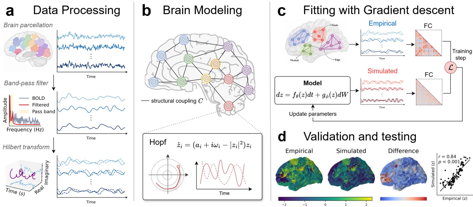
Figure 1:The workflow behind this notebook: (a) a brain scan is cut into regions and turned into signals, (b) every region becomes a small oscillator wired to the others, (c) the model is tuned until its simulated activity looks like the measured one, (d) the result is tested on new data.
Even when you lie still with your eyes closed, your brain is never quiet: billions of neurons keep up slow, coordinated waves of activity that travel between brain regions. Can we write equations that reproduce this activity? And if we can, can we trust them enough to one day test a treatment on a virtual copy of a patient’s brain before trying it on the patient?
Our interactive notebook is an introduction to that question and to our recent work on hybrid models: equations that keep the physics we trust and let a neural network learn the part we do not know. You will:
- build a small virtual brain with our open-source package and watch it produce scanner-like signals;
- see how a real-valued brain signal is turned into a complex one (an amplitude and a rhythm);
- compute the fingerprint neuroscientists use most, functional connectivity;
- find out, with a three-line experiment, why the most obvious way of comparing a model with data fails;
- meet the three families of models (physics-based, data-driven and hybrid) and what they achieve on real brains.
Why model a brain?
A brain model is a set of equations whose solutions look like recorded brain activity. Once we have one, we can use it to
- understand — which ingredients (anatomy, rhythms, noise) are needed to explain what we see;
- diagnose — fitted model parameters can serve as markers that separate healthy and diseased brains;
- treat — test a stimulation protocol in silico on a “digital twin” of a patient before applying it [26].
For this to work, a model must satisfy three requirements that pull in different directions:
| Requirement | In plain words |
|---|---|
| Data fidelity | its simulated activity has the same statistics (“descriptors”) as the real brain |
| Interpretability | its parameters mean something to a neuroscientist, so the model can be trusted and checked |
| Personalisation | there is one model per person, trainable from the few recordings available for a single subject |
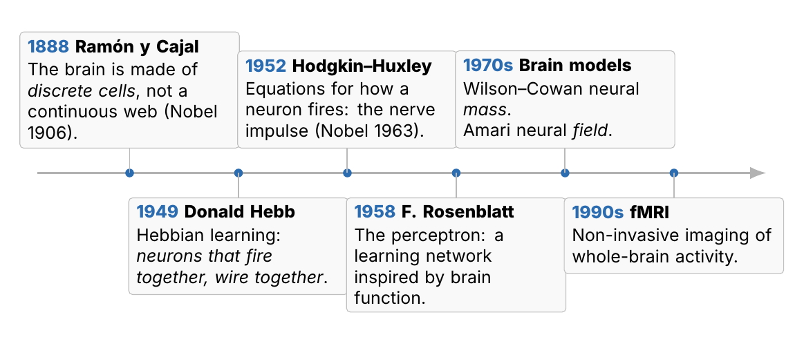
Figure 2: A century of brain models
Physics or machine learning? Three architectures
Traditional physics-based models of brain dynamics are interpretable and require little data, but their simplified assumptions limit their ability to reproduce complex neural activity. In contrast, fully data-driven models, such as Neural Stochastic Differential Equations, offer greater flexibility but require large datasets and are difficult to interpret.
The result is a model that balances physical interpretability, predictive flexibility, and data efficiency, with significantly fewer trainable parameters than a fully data-driven alternative.
| Coupled Physics | Neural SDE (data-driven) | |
|---|---|---|
| Data fidelity | ✗ too rigid | ✓ flexible |
| Data efficiency | ✓ few parameters | ✗ data hungry |
| Interpretability | ✓ physical model | ✗ black box |
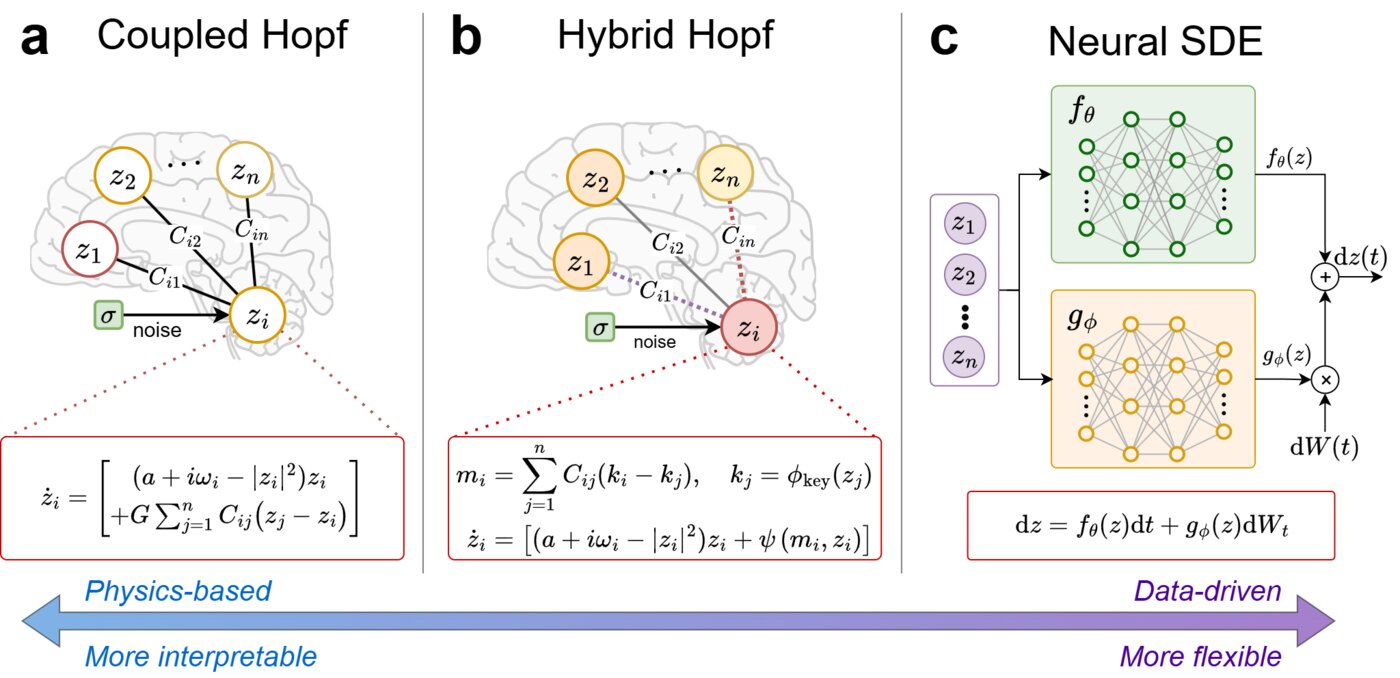
Figure 3:The three model families, from interpretable to flexible.
What happens with real brains
We trained the three models on resting-state fMRI from 94 subjects of the Human Connectome Project (100 regions), and evaluated them on held-out subjects.
| Model | FC corr ↑ | phase FC corr ↑ | FCD KS ↓ | phase FCD KS ↓ | metastability error ↓ | composite error ↓ |
|---|---|---|---|---|---|---|
| Coupled Hopf | 0.913 ± 0.011 | 0.783 ± 0.021 | 0.242 ± 0.009 | 0.208 ± 0.092 | 0.010 ± 0.005 | 0.189 ± 0.023 |
| Neural SDE | 0.787 ± 0.265 | 0.729 ± 0.329 | 0.145 ± 0.133 | 0.217 ± 0.065 | 0.037 ± 0.047 | 0.211 ± 0.163 |
| Hybrid Hopf | 0.926 ± 0.010 | 0.923 ± 0.014 | 0.100 ± 0.019 | 0.101 ± 0.041 | 0.010 ± 0.005 | 0.088 ± 0.010 |
Mean ± standard deviation over 10 independent trainings. “corr” is the correlation between simulated and empirical matrices (higher is better); “KS” is the Kolmogorov–Smirnov distance between distributions (lower is better); the composite error averages the four core descriptors.
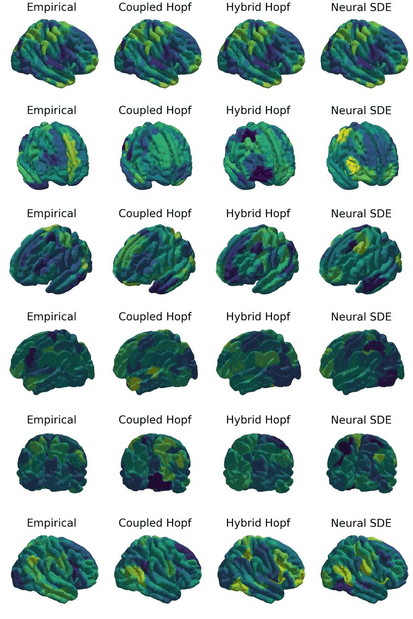
Figure 4: Brain activity painted on the cortex, for a real recording and for the three trained models.
The physics-based model is stable but cannot reproduce phase relations and dynamics. The Neural SDE is flexible but unreliable: some trainings fail completely, which explains its large spread. The hybrid model is the only one that is both accurate and reproducible, while keeping an oscillator whose parameters still have a meaning. In summary:
| Coupled Hopf | Hybrid Hopf | Neural SDE | |
|---|---|---|---|
| Reproduces network structure (FC, phase FC) | ∼ partly | ✓ | ∼ unstable across trainings |
| Reproduces network dynamics (FCD, phase FCD) | ✗ | ✓ | ∼ partly |
| Interpretable parameters | ✓ | ✓ | ✗ |
| Uses the anatomical connectome | ✓ | ✓ | ✗ |
| Works with little data (10 subjects) | ✓ | ✓ | ✗ |
| Captures the individual (1 subject) | ✗ | ✓ | ✓ |
| Learnable parameters | 2 | ≈ 2 200 | ≈ 220 000 |
Open questions
- Many objectives at once. The loss picks one point on a Pareto front of trade-offs between descriptors. Which point should we pick, and can we explore the whole front?
- Control. The clinical goal is stimulation: add an input to the drift and ask whether the brain can be steered (controllability), with which protocol (optimal control), and with feedback in closed loop.
- From regions to neurons and back. As the number of neurons goes to infinity, mass models should reconnect to the neural field equations they came from. What does the learned system do as?