Model Predictive Control with Random Batch Method for Linear-Quadratic Optimal Control: Introduction and Matlab Implementation
Spain. 02.05.2022
Author: Alexandra Borkowski
Optimal Control Problems in Practice
Imagine that you are given a new project at work that you shall complete successfully within a time T; how would you approach this task? As a mathematician, you may see this task as an Optimal Control Problem, i.e. you would try to get your optimal work input \bm{u}^*(t) which minimizes the functional
J(\bm{x}(t),\bm{u}(t)) = \frac{1}{2} \int_0^{T} L(\bm{x}(t), \bm{u}(t), t)\,dt, (1)
where L(\bm{x}(t), \bm{u}(t), t) denotes the ongoing cost rate of the project, e.g. the daily investments done by your company or your daily workload. The involved variable \bm{x}(t) can be seen as the actual work output from your project and it may be connected to your work input u(t) through some dynamics
\dot{\bm{x}}(t) = f(\bm{x}(t), \bm{u}(t), t) \qquad \bm{x}(0) = \bm{x}_0, (2)
which acts as a constraint in the minimization of J(\bm{x}(t),\bm{u}(t)). We are particularly interested in the the optimal work output \bm{x}^{*}(t) which result from the optimal work input \bm{u}^{*}(t):
\dot{\bm{x}}^{*}(t) = f(\bm{x}^{*}(t), \bm{u}^{*}(t), t) \qquad \bm{x}^{*}(0) = \bm{x}_0. (3)
The longer the planning horizon T, the trickier it seems to get the optimal work input (or optimal control) \bm{u}^{*}(t), right?
In this blog post, we want to explore how the optimal work output (or optimal trajectory) \bm{x}^{*}(t) can be approximated in the case of long time horizons by the RBM-MPC Strategy, which combines Model Predictive Control (MPC) and the Random Batch Method (RBM). This strategy repetitively predicts an optimal control for reduced dynamics and subsequently applies it to the dynamics. It was first suggested by Ko and Zuazua [2021] when they considered an Optimal Control Problem for a non-linear and multi-agent dynamical system. For the ease of understanding (and upcoming convergence analyses), we opt to consider a simpler Optimal Control Problem though, which we introduce in the following. We then discuss MPC and the RBM in this setting and join the two approaches subsequently to the RBM-MPC strategy. Finally, we show a numerical example for a one-dimensional wave equation which is discretized by finite differences.
Linear-Quadratic Optimal Control
We consider an infinite time horizon and a Linear-Quadratic Optimal Control, i.e. the cost rate is quadratic both in the state variable \bm{x}_{\infty}(t) and the control variable \bm{u}_{\infty}(t) and its computed over 0 \to \infty:
J_{\infty}(\bm{u}_{\infty}) = \frac{1}{2} \int_0^{\infty} \bm{x}_{\infty}(t)^TQ\bm{x}_{\infty}(t) + \bm{u}_{\infty}(t)^TR\bm{u}_{\infty}(t)\,dt. (4)
Furthermore, \bm{x}_{\infty}(t) and \bm{u}_{\infty}(t) are dynamically connected through the linear time invariant system
\dot{\bm{x}}_{\infty}(t) = A\bm{x}_{\infty}(t) + B\bm{u}_{\infty}(t), \bm{x}_{\infty}(0) = \bm{x}_0. (5)
We further assume \bm{x}_{\infty}(t) \in L^2([0,\infty);\mathbb{R}^n), \bm{x}_0 \in \mathbb{R}^n, \bm{u}_{\infty}(t) \in L^2([0,\infty);\mathbb{R}^q), A \in \mathbb{R}^{n\times n}, Q \in \mathbb{R}^{n\times n}, B \in \mathbb{R}^{n \times q} and R \in \mathbb{R}^{q\times q}. Moreover, R is positive definite and Q is positive semi-definite and the pair (A,B) is assumed to be controllable. We are thus interested in approximating the solution \bm{x}_{\infty}^{*}(t) of
\dot{\bm{x}}_{\infty}^{*}(t) = A\bm{x}_{\infty}^{*}(t) + B\bm{u}_{\infty}^{*}(t), \bm{x}_{\infty}^{*}(0) = \bm{x}_0. (6)
How do we approximate \bm{x}_{\infty}^{*} ?
Predict and Synchronize: Model Predictive Control
The first main idea is that we approximate the infinite-horizon trajectory \bm{x}_{\infty}^*(t) with many finite-horizon trajectories, i.e. we repetitively predict an optimal control over a time horizon T and subsequently apply it to the original dynamics for a time \tau \leq T. This approach corresponds to Model Predictive Control (MPC). MPC is often used in real-world problems when the true dynamics of a system are unknown, too complex, or influenced by noise. In these situations, MPC may enable control of the system nonetheless as the interplay of prediction over assumed dynamics and the reference back to the true system can outbalance uncertainties about the dynamics.
We denote \tau_i := \tau i, i \geq 0, in the following. Starting at i = 0, we predict over [\tau_0, \tau_0 + T], and obtain an optimal control u^*_{T}(t), which minimizes
J_{T,\,\tau_0}(\bm{u}_{T}) = \int_{\tau_{0}}^{\tau_{0} + T} \Bigg(\bm{x}_{T}(t)^TQ\bm{x}_{T}(t) + \bm{u}_{T}(t)^TR\bm{u}_{T}(t)\Bigg)\,dt, (7)
where \bm{x}_{T}(t) fulfills
\dot{\bm{x}}_{T}(t) = A\bm{x}_{T}(t) + B\bm{u}_{T}(t), \bm{x}_{T}(0) = \bm{x}_0. (8)
We now apply \bm{u}_T^* to the true dynamics and obtain like this the state \bm{x}^*_{T}
\dot{\bm{x}}^*_{T}(t) = A\bm{x}^*_{T}(t) + B\bm{u}^*_{T}(t), \bm{x}^*_{T}(0) = \bm{x}_0, (9)
which we set to the MPC trajectory \bm{x}^*_{M} on t \in [0, \tau_1]. This procedure is repeated: Starting from the state \bm{x}_{M}^*(\tau_1), we predict the randomized control \bm{u}_T^* over [\tau_1, \tau_1 + T] and apply it to the system over [\tau_1, \tau_1 + T], which yields \bm{x}_{T}^* on [\tau_1, \tau_2]. Note that \bm{u}_T^* and \bm{x}_{T}^* depend on \bm{x}_{M}^*(\tau_1). We proceed like this until we exceed some given maximum time scale T_{\text{max}}, i.e. until \tau_i + T \leq T_{\text{max}}. The MPC procedure is illustrated in Figure 1 and can be summarized as follows:
1- Initialize the state: \bm{x}^*_{M}(0) = \bm{x}_0, i = 0.
2- While \tau_{i} + T \leq T_{\text{max}}:
a) Compute \bm{u}_T^{*}(t,\bm{x}^{\tau_i}_{M}) on [\tau_i, \tau_i + T].
b) Determine \bm{x}_{T}^{*}(t,\bm{x}^{\tau_i}_{M}) on [\tau_i, \tau_{i+1}] by solving
\dot{\bm{x}}^*_{T}(t,\bm{x}^*_{M}(\tau_i)) = A\bm{x}^*_{T}(t,\bm{x}^*_{M}(\tau_i)) + B\bm{u}_T^{*}(t,\bm{x}^*_{M}(\tau_i)) \bm{x}^*_{T}(\tau_i,\bm{x}^*_{M}(\tau_i)) = \bm{x}^*_{M}(\tau_i).
c) Set \bm{x}_M^*(t) = \bm{x}^*_{T}(t,\bm{x}^*_{M}(\tau_i)) on [\tau_i, \tau_{i+1}].
d) i = i + 1.
In this setting, two time scales arise. First, the prediction horizon T and second, the shorter control or synchronization time \tau. Intuitively, the MPC strategy will approximate \bm{x}^*_{\infty} well when T is chosen to be sufficiently long and \tau is chosen to be sufficiently short.
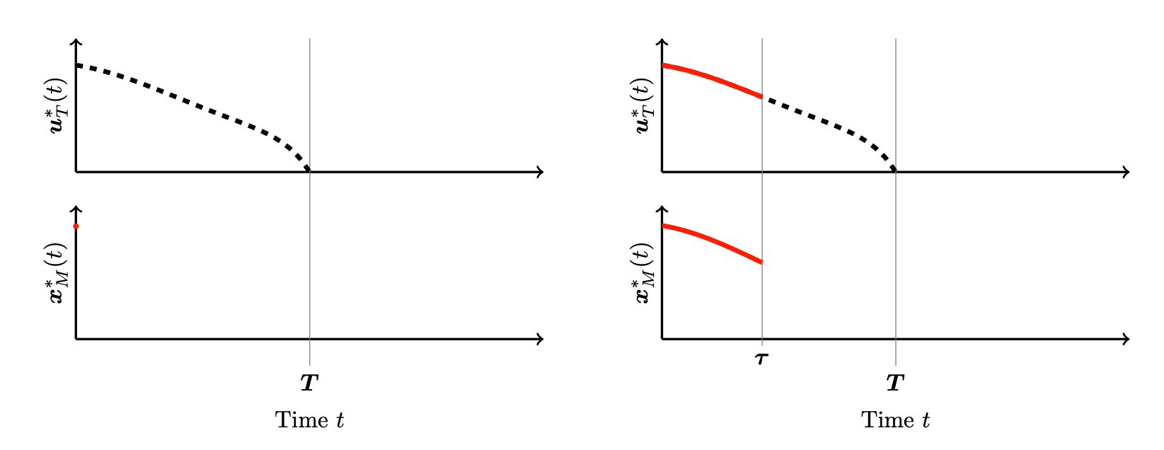
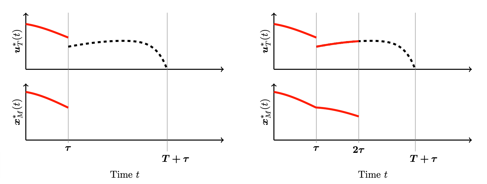
Figure 1. Illustration of the MPC strategy (courtesy of Daniël Veldman). The dashed black line represents the prediction of the future control over a time horizon of length T. This prediction is then applied over a shorter time horizon of length \tau = \tau_{i+1} - \tau_i, represented by the red line for both the control \bm{u}_T^*(t) and state \bm{x}_M^*(t).
Reduce Computational Cost: The Random Batch Method
By computing many finite-horizon trajectories \bm{x}_{T}^*, we increase the computational demand. This gives rise to another idea: We simplify the dynamics. For linear dynamics, this may mean that we replace A with – potentially – sparser matrices and compute the optimal control for these reduced dynamics \bm{u}^*_R. These reduced dynamics shall still approximate the true dynamics sufficiently, nonetheless. Therefore, one may use the following approach suggested in Veldman and Zuazua [2022]:
• Decompose the matrix A as
A = \sum_{m=1}^M A_m.
E.g.: For M=2, this means A = A_1 + A_2.
• Enumerate the 2^M subsets of \{1,2,\ldots,M \} as S_1, S_2, \ldots, S_{2^M} and assign to each subset S_\omega a probability p_\omega such that \sum_{\omega=1}^{2^M} p_\omega = 1.
E.g.: S_1=\{A_1\}, S_2=\{A_2\}, S_3 = \{A_1, A_2\}, S_4 = \emptyset, with p_1 = p_2 = p_3 = p_4 = \frac{1}{4}.
• Divide [0{,}\,T] into K subintervals [t_{k-1},t_k) of length h.
For each [t_{k-1},t_k), randomly choose an index \omega_k \in \{1,2, \ldots , 2^M \} according to the probabilities p_{\omega}. Set \boldsymbol \omega = (\omega_1, \omega_2, \ldots, \omega_K). E.g.:
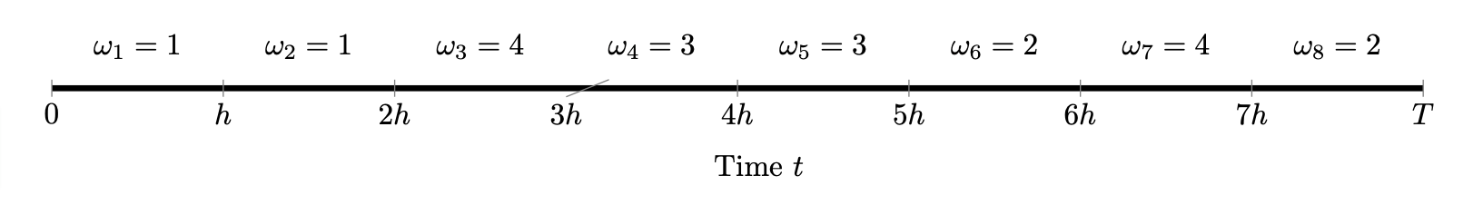
• Define the mapping t \mapsto A_h(\bm{\omega}, t)
A_h(\bm{\omega}, t) = \sum_{m \in S_{\omega_k}} \frac{A_m}{\pi_m}, \qquad \qquad t \in [t_{k-1}, t_k),
where \pi_m is the probability that m is an element of the selected subset, i.e.
\pi_m = \sum_{\omega \in \{ \omega \mid m \in S_\omega \} } p_\omega,
E.g.: A_h(\bm{\omega}, t) = 2A_1, for t \in [0,2h), A_h(\bm{\omega}, t) = 2A_1+2A_2 = 2A, for t \in [2h,3h), …
• Compute the minimizer \bm{u}_R^*(\bm{\omega}, t) of the simpler problem
\min_{\bm{u}_R \in L^2(0{,}T; \mathbb{R}^q)} J_R(\boldsymbol \omega, \bm{u}) = \int_0^T \left( \bm{x}_R(\bm{\omega}, t)^T Q \bm{x}_R(\bm{\omega}, t) + \bm{u}_R(t)^T R \bm{u}_R(t) \right) dt,
\dot{\bm{x}}_R(\bm{\omega}, t) = \textcolor{orange}{A_h(\bm{\omega}, t)}\bm{x}_R(\bm{\omega}, t) + B\bm{u}_R(t),\;\;\;\;\bm{x}_R(\bm{\omega}, 0) = \bm{x}_0.
Since the selection of the value of A_h at time t is randomized and since the matrices A_m correspond to certain batches of the components of the state variable, \bm{x}_R, this strategy can be seen as a Random Batch Method (RBM).
Let’s mix it up: Model Predictive Control with Random Batch Method
The combination of MPC and the RBM, gives rise to the following RBM-MPC strategy:
1- Initialize the state: \bm{x}^*_{R-M}(0) = \bm{x}_0, i = 0; \Omega_{-1} = \emptyset
2- While \tau_{i} + T \leq T_{\text{max}}:
a) Fix \bm{\omega} \in \{1,2,\dots,2^M\}^K according to the probabilities \{p_{\omega}\}_{{\omega}=1}^{2^M}
b) Compute \bm{u}_R^{*}(\bm{\omega},t,\bm{x}^*_{R-M}(\Omega_{i-1},\tau_i)) on [\tau_i, \tau_i + T]
c) Determine \bm{x}_{T}^{*}(\bm{\omega}, t,\bm{x}^*_{R-M}(\Omega_{i-1},\tau_i)) on [\tau_i, \tau_{i+1}] by solving
\dot{\bm{x}}^*_{T}(\bm{\omega},t,\bm{x}^*_{R-M}(\Omega_{i-1},\tau_i)) = A\bm{x}^*_{T}(\bm{\omega},t,\bm{x}^*_{R-M}(\Omega_{i-1},\tau_i)) + B\bm{u}_R^{*}(\bm{\omega}, t,\bm{x}^*_{R-M}(\Omega_{i-1},\tau_i))
\bm{x}^*_{T}(\bm{\omega},\tau_i,\bm{x}^*_{R-M}(\Omega_{i-1},\tau_i)) = \bm{x}^*_{R-M}(\Omega_{i-1},\tau_i)
d) \bm{x}_{R-M}^*(\bm{\omega},\Omega_{i-1},t) = \bm{x}^*_{T}(\bm{\omega}_i,t,\bm{x}^*_{R-M}(\Omega_{i-1},\tau_i)) on [\tau_i, \tau_{i+1}].
e) \Omega_{i-1} = \{\Omega_{i-1}, \bm{\omega}\}
f) i = i + 1
In step (b) we compute \bm{u}_R^* over a time horizon of length T and implement it to the true dynamics in step (c) over a time \tau. This is repeated iteratively. Furthermore, we explicitly collect the previous selections of \bm{\omega} in the set \Omega_{i-1} to acknowledge the fact that \bm{x}^*_{R-M} at time t depends on all those previous selections.
Note that the RBM-MPC strategy can also be motivated by the following viewpoint (following Ko and Zuazua [2021]): Whenever we have non-linear, high-dimensional dynamics, the computation of an optimal control \bm{u}_T^* can be costly as the Gradient Descent Method requires the evaluation of the full state equation and adjoint system in each iteration, which may consist in numerous interaction terms. Thus, the RBM, which only takes into account interactions within random batches, can be introduced to decrease the computational cost. However, the optimal controls of the reduced and the original system, \bm{u}_R^* and \bm{u}_T^* (or \bm{u}_{\infty}^*), will generally not coincide. The additional introduction of MPC can compensate for arising errors and lead to an efficient and converging algorithm.
RBM-MPC in Practice
Pseudocode for the time-continuous RBM-MPC with Gradient Descent
The previously stated RBM-MPC algorithm does not specify the computation of the randomized control \bm{u}_R^*(\bm{\omega},t). In practice, we may compute \bm{u}_R^*(\bm{\omega},t) with the Gradient Descent Method for the functional J_R(\bm{\omega}, \bm{u}_R). By considering the Gâteaux derivative of the corresponding Lagrangian, the gradient of J_R can be shown to be R\bm{u}_R + B^T\bm{\phi}_R, where \bm{\phi}_R denotes the adjoint state, which was introduced as a Lagrangian multiplier.
This leads to the following, adapted pseudocode of the RBM-MPC combined with Gradient Descent:
1- Initialize the state: \bm{x}^*_{R-M}(0) = \bm{x}_0, i = 0
2- While \tau_{i} + T \leq T_{\text{max}}:
a) Initialize the control: \bm{u}_R^0(t) = \bm{u}_R(t), n = 0
b) Fix \bm{\omega} \in \{1,2,\dots,2^M\}^K according to the probabilities \{p_{\omega}\}_{\omega=1}^{2^M}
c) While convergence criterion is not fulfilled do
i. Determine \bm{x}_R(\bm{\omega},t) on [\tau_i,\tau_i + T] by solving
\dot{\bm{x}}_R(\bm{\omega},t) = A_h(\bm{\omega},t)\bm{x}_R(\bm{\omega},t) + B\bm{u}_R^n(\bm{\omega},t),
\bm{x}_R(\bm{\omega},\tau_i) = \bm{x}^{*}_{R-M}(\tau_i)
ii. Determine \bm{\phi}_R(\bm{\omega}, t) on [\tau_i,\tau_i + T] by solving
-\dot{\bm{\phi}}_R(\bm{\omega},t) = A_h^T(\bm{\omega},t)\bm{\phi}_R(\bm{\omega},t) + Q\bm{x}_R(\bm{\omega},t)
\bm{\phi}_R(\bm{\omega},\tau_i+T) =0
iii. Update Control using Gradient Descent:
\bm{u}_R^{n+1}(\bm{\omega},t) = \bm{u}_R^{n}(\bm{\omega},t) - \alpha (B^T\bm{\phi}_R(\bm{\omega},t) + R\bm{u}_R^n(\bm{\omega},t))
iv. n = n + 1
d) Determine \bm{x}^*_{R-M}(\bm{\omega},t) on [\tau_i, \tau_{i+1}] by solving
\dot{\bm{x}}^*_{R-M}(\bm{\omega},t) = A\bm{x}^*_{R-M}(\bm{\omega},t) + B\bm{u}_R^{n+1}(\bm{\omega},t) \bm{x}^*_{R-M}(\bm{\omega},\tau_i) = \bm{x}^{*}_{R-M}(\tau_i)
3- i = i + 1
We choose \frac{|J_R(\bm{u}_R^{n})) - J_R(\bm{u}_R^{n-1})|}{J_R(\bm{u}_R^{n-1})} \leq 10^{-5} as our convergence criterion but also other choices are possible. We further omitted the explicit dependence on previous choices of \bm{\omega} in the above pseudo-code for readability.
RBM-MPC for the 1-D Wave Equation
We now consider the one-dimensional wave equation on a string, described by the spatial domain \Omega = [0,L], and for times 0 \leq t \leq T. The vertical deflection of the string is denoted by s: \Omega \times [0,T] \rightarrow \mathbb{R}. For all times t > 0, the deflection of the string is described by the wave equation:
\frac{\partial^2 s}{\partial t^2} = c^2 \frac{\partial^2 s}{\partial x^2},\;\;\;\forall\, (x,t) \in (0,L)\times (0,T]. (10)
At time t = 0, the string is at rest, but deflected in the following way:
s(x,0) = 3\sin(\frac{\pi x}{L}), \forall\, x \in \Omega \frac{\partial}{\partial t} s(x,t)|_{t = 0} = 0, \forall\, x \in \Omega (11)
We further impose the Neumann boundary conditions at the ends of the string, meaning that the boundaries are reflective:
\frac{\partial}{\partial x}s(0,t) = 0, \forall\, t \in [0,T] \frac{\partial}{\partial x}s(L,t) = 0, \forall\, t \in [0,T]. (12)
To use our described RBM-MPC strategy, we want to cast the wave equation into a linear system and thus discretize it in space, meaning that we select N_x nodes on the string, which divide it into N_x-1 pieces of length L/(N_x-1)=:\Delta x. Denoting with s_j the deflection at the node j, j = 1, \dots, N_x, we can approximate the spatial Laplacian by
\frac{\partial^2 s_j(t)}{\partial x^2} \approx \frac{s_{j-1}(t) - 2s_{j}(t)+s_{j+1}(t)}{\Delta x^2}. (13)
To discretize according at j = 1 and j = N_x, ghosts points s_0(t) and s_{N_x+1}(t) would have to be introduced but due to the Neumann conditions
\frac{s_2(t) - s_0(t)}{2\Delta x} = 0 (14)
and
\frac{s_{N_x+1}(t) - s_{N_x-1}(t)}{2\Delta x} = 0 (15)
we see that their values just correspond to s_2(t) and s_{N_x-1}(t), respectively. Plugging these considerations into the wave equation yields
\begin{pmatrix} \frac{\partial^2}{\partial t^2}s_{1}(t) \\ \frac{\partial^2}{\partial t^2}s_{2}(t) \\ \dots \\ \frac{\partial^2}{\partial t^2}s_{Nx-1}(t) \\ \frac{\partial^2}{\partial t^2}s_{Nx}(t) \\ \end{pmatrix} = \underbrace{\frac{c^2}{\Delta x^2} \begin{pmatrix} -2 & 2 & & \\ 1 & -2 & 1 & \\ & & \ddots & \\ & 1& -2& 1 \\ & & 2 & -2 \end{pmatrix}}_{c^2\Delta_D} \begin{pmatrix} s_{1}(t) \\ s_{2}(t) \\ \dots \\ s_{Nx-1}(t) \\ s_{Nx}(t) \end{pmatrix}. (16)
To cast the equation into a linear equation of the form
\dot{\bm{x}}_T(t) = A\bm{x}_T(t), (17)
we further introduce
\bm{x}_T(t)=\begin{pmatrix} s_1(t) \\ \dots \\ s_{N_x}(t) \\ \dot{s}_1(t) \\ \dots \\ \dot{s}_{N_x}(t) \end{pmatrix}. (18)
This allows us to write
\dot{\bm{x}}_T(t) = \begin{pmatrix} 0_{N_x, N_x} & I_{N_x, N_x} \\ c^2\Delta_D & 0_{N_x, N_x} \end{pmatrix}\bm{x}_T(t). (19)
Now, we also add a control force u_T(t) \in L^2([0,T];\mathbb{R}) to the wave equation:
\frac{\partial^2 s(x,t)}{\partial t^2} = c^2 \frac{\partial^2 s(x,t)}{\partial x^2} + \delta(x-L)u_T(t). (20)
Here, the force only acts on the right boundary of the string. By defining B = (0,\dots,0,1)^T \in \mathbb{R}^{N_x}, we can write the spatially discretized wave equation in our linear standard form \dot{\bm{x}_T}(t) = A\bm{x}_T(t) + B\bm{u}_T(t):
\dot{\bm{x}}_T(t) = \begin{pmatrix} 0_{N_x, N_x} & I_{N_x, N_x} \\ c^2\Delta_D & 0_{N_x, N_x} \end{pmatrix}\bm{x}_T(t) + \begin{pmatrix} 0 \\ \vdots \\ 0 \\ 1 \end{pmatrix}u_T(t). (21)
We choose our cost functional J_T:L^2([0, T];\mathbb{R})\rightarrow\mathbb{R} as
J_T(u_T(t)) = \int_0^T |\bm{x}_T(t)|^2 + |u_T(t)|^2\;dt, (22)
i.e. we set Q = I_{2N_x, 2N_x} and R=1 in the general form of the cost functional.
In our example, we set N_x=11 and decompose the matrix A as
A = \begin{pmatrix} 0_{N_x, N_x} & I_{N_x, N_x} \\ c^2\Delta_D & 0_{N_x, N_x} \end{pmatrix} = \underbrace{\begin{pmatrix} 0_{N_x, N_x} & \frac{1}{2}I_{N_x, N_x} \\ c^2\Delta_{D,1} & 0_{N_x, N_x} \end{pmatrix}}_{A_1} + \underbrace{\begin{pmatrix} 0_{N_x, N_x} & \frac{1}{2}I_{N_x, N_x} \\ c^2\Delta_{D,2} & 0_{N_x, N_x} \end{pmatrix}}_{A_2}, (23)
with
\Delta_{D,1} = \frac{1}{\Delta x^2} \begin{pmatrix} -2 & 2 & & & & & & \\ 1 & -2 & 1 & & & & & \\ & & \ddots & & & & & \\ & & 1 & -2 & 1 & & & & \\ & & & 1 & -1 & 0 & & & \\ & & & & 0 & 0 & 0 & & \\ & & & & & & \ddots & & \\ & & & & & 0 & 0 & 0 & \\ & & & & & & & 0 & 0 \end{pmatrix} (24)
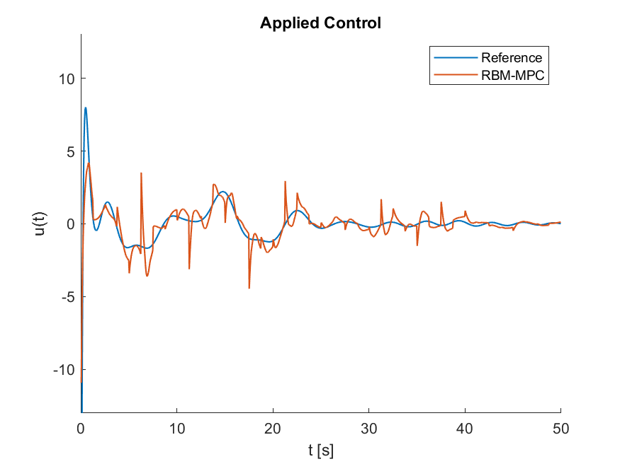
Figure 2. The optimal control \bm{u}^*_{\infty} is displayed in blue and the randomized control \bm{u}^*_{R} in orange.
and
\Delta_{D,2} = \frac{1}{\Delta x^2} \begin{pmatrix} 0 & 0 & & & & & & \\ 0 & 0 & 0 & & & & & \\ & & \ddots & & & & & \\ & & 0 & 0 & 0 & & & & \\ & & & 0 & -1 & 1 & & & \\ & & & & 1 & -2 & 1 & & \\ & & & & & & \ddots & \\ & & & & & & 1 & -2 &1 \\ & & & & & & & 2 & -2 \end{pmatrix}. (25)
To the subsets \{A_1\} and \{A_2\}, we assign each a possibility of \frac{1}{2} and to the subsets \{A_1, A_2\} and \emptyset the probability 0.
The only task left is now the choice of time discretization. We opt for a discretize-then-optimize strategy, i.e. we discretize the cost functional and obtain discretized versions of the state and adjoint equations by solving the sufficient conditions of the Lagrangian. In particular, we discretize the functional J_R(\bm{\omega},\bm{u}_R) by the trapezoidal rule in the state part and by the midpoint rule in the control part and choose to solve the state equation with a Crank Nicolson scheme; the details can be seen from the attached code but also Apel and Flaig [2012] is a very insightful reference.
Using the attached code, which implements the RBM-MPC strategy in the above described manner, yields the trajectory and the applied control displayed in the Video below and in Figure 2. Here, we chose T_{max} = 50 sec, T = 10 sec, \tau = 1.25 sec, and h = 0.05 sec. The reference trajectory control in blue corresponds to \bm{x}_{\infty}^*(t) and \bm{u}^*_{\infty}, respectively, which were computed by Matlab’s LQR-function from its Control System Toolbox.
References
• T. Apel and T. G. Flaig. Crank–nicolson schemes for optimal control problems with evolution equations. SIAM Journal on Numerical Analysis, 50(3):1484–1512, 2012.
• D. Ko and E. Zuazua. Model predictive control with random batch methods for a guiding problem. Mathematical Models and Methods in Applied Sciences, 31(08):1569–1592, 2021.
• D.W.M. Veldman and E. Zuazua. A framework for randomized time-splitting in linear-quadratic optimal control (2022) Numerische Mathematik. DOI: https://doi.org/10.1007/s00211-022-01290-3