PDF poster… | Download Code… | Related Paper…
The problem
 Control of a parameter dependent system in a robust manner.
Fix a control time $T > 0$, an arbitrary initial data $x^0$, and a final target $x^1 \in R^N$
Given $\varepsilon > 0$ we aim at determining a family of parameters $\nu_1,…, , \nu_n$ in $\mathcal{N}$ so that the corresponding controls $u_1, …, u_n$ are such that for every $\nu \in \mathcal{N}$ there exists $u^\star_\nu \in {\rm span}\{u_1,…, u_n\}$ steering the system to the state $x_\nu^\star(T)$ within the $\varepsilon$ distance from the target $x^1$.
The system
A finite dimensional linear control system:
\begin{equation}\begin{cases}
x'(t)=A( \nu)x(t)+Bu(t),\,0 < t < T,\\ x(0)=x^0 \end{cases} \end{equation} [/latex]
- $ A( \nu)$ is a $N \times N$−matrix,
- $B$ is a $N\timesM$ control operator, $\,M \leq N$,
- $\nu$ is a parameter living in a compact set, $\,\mathcal{N}$ of $\mathbb{R}^d$
Assumptions:
- the system is (uniform) controllable for all $\nu \in N$,
- system dimension $\mathcal{N}$ is large
The greedy approach
$X$ -- a Banach space
$K\subset X$ -- a compact subset.
The method approximates $K$ by a a series of finite dimensional linear spaces $V_n$ (a linear method).
A general greedy algorithm
- The first step Choose $x_1 \in K$ such that $$ {{\| x_1 \|}_{X}} = \max_{x \in K} {{\| x \|}_{X}} $$
- The general step Having found $x_1 .. x_n$, denote $$ V_n={\rm span} \{x_1, \ldots,x_n\} $$ Choose the next element $$ x_{n+1}:= \arg\!\max_{x \in K} {\rm dist}(x, V_n)\, $$
- The algorithm stops When $\crv{\sigma_n(K)}:= \max_{x \in K} {\rm dist}(x, V_n) $ becomes less than the given tolerance $\varepsilon$.
The Kolmogorov $n$ width, $d_n(K) $ measures optimal approximation of $K$ by a $n$-dimensional subspace.
$$
d_n(K):=\inf_{\dim Y=n} \sup_{x\in K} \, \inf_{y\in Y} {{\| x-y \|}_{X}}\,.
$$
The greedy approximation rates have same decay as the Kolmogorov widths.
Greedy control
Each control can be uniquely determined by the relation
$$
u_{\bf \nu} = {\bf B}^\ast e^{(T-t){\bf A}_{\bf \nu}^\ast} \varphi^0_{\bf \nu},
$$
where $\varphi^0_{\bf \nu}\in {{\bf R}}^N$ is the unique minimiser of a quadratic functional associated to the adjoint problem.
This minimiser can be expressed as the solution of the linear system
\begin{equation*}
\label{phi^0}
\Lambda_{\bf \nu} \varphi^0_{\bf \nu} = {\sf x}^1 - e^{T{\bf A}_{\bf \nu}} {\sf x}^0,
\end{equation*}
where $\Lambda_{\bf \nu} $ is the controllability Gramian
\begin{equation*}
\Lambda_{\bf \nu}=\int_0^T e^{(T-t){\bf A}_{\bf \nu}}{\bf B}_{\bf \nu} {\bf B}_{\bf \nu}^\ast e^{(T-t){\bf A}_{\bf \nu}^\ast} dt\,.
\end{equation*}
Perform a greedy algorithm to the manifold $\varphi^0({\cal N})$:
$$
\nu \in {\cal N} \to \varphi^0_\nu \in \bf{R}^N\,.
$$
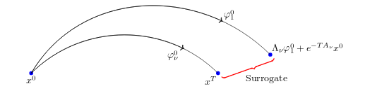
The (unknown) quantity ${\rm dist} (\varphi^0_{\bf \nu}, \varphi_i^0)$ to be maximised by the greedy algorithm is replaced by a surrogate:
$$
\begin{aligned}
{\rm dist} (\varphi^0_{\bf \nu}, \varphi_i^0)
&\sim {\rm dist} (\Lambda_{\bf \nu} \varphi^0_{\bf \nu}, \Lambda_{\bf \nu} \varphi^0_i) \cr
&= {\rm dist} ({\sf x}^1 - e^{T{\bf A}_{\bf \nu}} {\bf x}^0, \Lambda_{\bf \nu} \varphi^0_i) \,.\cr
\end{aligned}
$$

The greedy control algorithm results in an optimal decay of the approximation rates.
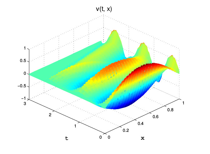
Numerical examples
Wave equation
We consider the system (1) with:
$$
{\bf A}=\left(\begin{matrix}
{\bf 0} & -I\cr
{ \nu} ( N/2+1)^2 \tilde {\bf A} & {\bf 0}\cr
\end{matrix}\right),
$$
$$
\tilde {\bf A}=\left(\begin{matrix}
2 & -1& 0 & \cdots & 0\cr
-1& 2 & -1& \cdots & 0\cr
0 & -1& 2 & \cdots & 0\cr
\vdots&\vdots&\vdots&\ddots&\vdots\cr
0 &0& 0 & \cdots &2\cr
\end{matrix}\right),
\quad
{\bf B}=\left(\begin{matrix}
0\cr
0\cr
\vdots\cr
0\cr
1\cr
\end{matrix}\right).
$$
The system corresponds to the discretisation of the wave equation problem with the control on the right boundary:
\begin{equation}
\left\{
\begin{split}
\partial_{tt} v - \crven{\nu} \partial_{xx} v&=0, \qquad (t, x) \in {\langle#0,#T\rangle} \times {\langle#0,#1\rangle} \\
v(t, 0)=0, &\quad v(t, 1)=u(t)\\
v(0, x)=v_0,& \quad \partial_t v(x, 0)=v_1\,.\\
\end{split
}
\right.
\end{equation}
We take the following values:
$$T=3,\; N=50,\;
v_0=\sin(\pi x), \; v_1=0,\;
x^1=0
$$
$$
\nu \in {[#1,#10]} = {\cal N}
$$
The greedy control has been applied with $\varepsilon=0.5$ and the uniform discretisation of ${\cal N}$ in $k=100$ values.
The offline algorithm stopped after 24 iterations.
The 20-D controls manifold is well approximated by a 10-D subspace:
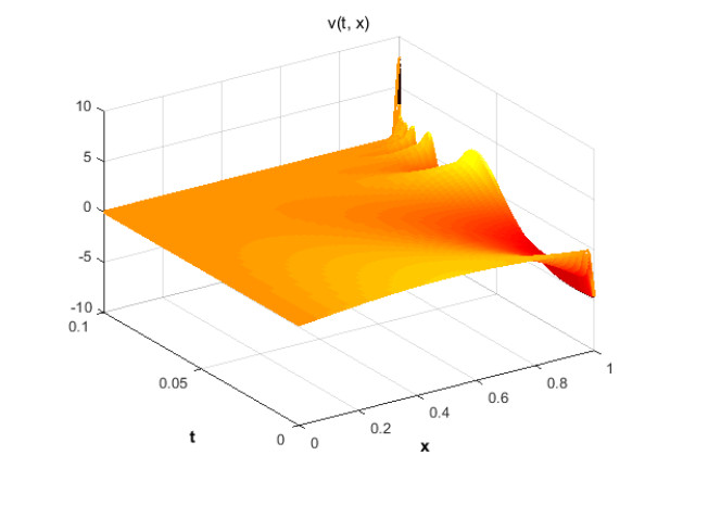
Heat equation
For $ {\bf A}=( N+1)^2\tilde{\bf A} $, with $\tilde{\bf A}$ given by:
$$
\tilde {\bf A}=\left(\begin{matrix}
2 & -1& 0 & \cdots & 0\cr
-1& 2 & -1& \cdots & 0\cr
0 & -1& 2 & \cdots & 0\cr
\vdots&\vdots&\vdots&\ddots&\vdots\cr
0 &0& 0 & \cdots &2\cr
\end{matrix}\right)
$$
and the control operator $ {\bf B}= (0, \ldots,0, ( N+1)^2 )^\top,$ the system (1) corresponds to the space-discretisation of the heat equation problem with $N$ internal grid points and the control on the right boundary:
\begin{equation}
\left\{ \begin{split}
\partial_{t} v - \nu \partial_{xx} v&=0, \qquad (t, x) \in {\langle#0,#T\rangle} \times {\langle#0,#1\rangle},\\
v(t, 0)&=0, \quad v(t, 1)=u_\nu(t),\\
v(0, x)&=v_0.\\
\end{split}\right.
\end{equation}
The parameter $\nu$ represents the diffusion coefficient and is supposed to range within the set ${\cal N}={[#1,#2]}$.
The system satisfies the Kalman's rank condition for any $\nu\in {\cal N}$ and any target time $T$.
We aim to control the system from the initial state $v_0(x)=\sin(\pi x)$ to zero in time $T=0.1$.
The greedy control algorithm has been applied for the system of dimension $N=50$ with $\varepsilon=0.0001$, and the uniform discretisation of ${\cal N}$ in $k=100$ values.
The algorithm stops after only three iterations.

MATLAB CODE
Below you can see and download the MATLAB code executed to simulate and to obtain the data results related to the Greedy control problem. That code is divided into two main files, corresponding to the offline algorithm and the online algorithm respectively, and several additional functions used by both algorithms.
The Offline Algorithm
%% initiation

clear f A B y par_greedy sigma G G_nu_phi0 rhs phi0_sel nu_sel;
N=20; %system dimension
k=100; %discretisation constant of a parameter set

x0=zeros(N,1); %initiation of the initial condition

if 0 %wave eq. setting
    cc=1; %example number
    nt=10*N;  %discretisation of the time interval
    a=1; b=10; %parameter interval
    d_nu=(b-a)/k;
    nu=a:d_nu:b;
    n= size(nu,2)-1;
    T=3; %target time
    epsil=0.5; % greedy control error
    %system matrix
    M=zeros(N/2);%N should be even
    I=eye(N/2);
    A_pom=2*eye(N/2);
    for i=1:1:N/2-1
        A_pom(i,i+1)=-1;
        A_pom(i+1,i)=-1;
    end
    A = zeros(N,N,n+1);
    for l=1:1:n+1
        A(:,:,l)=[M -I;  nu(l)*((N/2+1)^2)*A_pom  M];
    end
    %control operator
    B=zeros(N-1,1);
    B(N)=1*(N+1)^2;
    %initial condition
    for i=1:1:N/2
        x0(i)=1*sin(pi*(i)/(N/2+1));
    end
end

if 1 %heat eq. setting
    cc=2; %example number
    nt=30*N;  %discretisation of the time interval
    a=1; b=2; %parameter interval
    d_nu=(b-a)/k;
    nu=a:d_nu:b;
    T=0.1; %target time
    epsil=0.0001; %greedy control error
    %system matrix
    A = zeros(N,N,n+1);
    A_pom=2*eye(N);
    for i=1:1:N-1
        A_pom(i,i+1)=-1;
        A_pom(i+1,i)=-1;
    end
    for l=1:1:n+1
        A(:,:,l)=nu(l)*((N+1)^2)*A_pom;
    end
    %control operator
    B=zeros(N-1,1);
    B(N)=1*(N+1)^2;
    %initial condition
    for i=1:1:N
        x0(i)=1*sin(pi*(i)/(N+1));
    end
end

x1=0*ones(N,1); %target state

%% greedy control algorithm - offline part

k=N; %max. # of iterations
nu_iter=nu;

%Choosing the first parameter
y = zeros(k+1,1);
%calculation of free dynamics for all parameter values
for l=1:1:(k+1)
    x=sys_sol(x0,T,nt,-A(:,:,l), zeros(N,1), zeros(1,nt+1));
    rhs(:,l)=x1-x(:,nt+1);
    y(l)=norm(rhs(:,l)); %error in the first step
    if y(l)<epsil
        nu_iter(l)=0;
    end
end
%removing those parameter values for which we have already obtained
%approximation within a given error from further calculations
for l=size(nu_iter,2):-1:1
    if  nu_iter(l)==0
        nu_iter(l)=[];
    end
end
%selection of the first parameter
par_greedy(1)=argmax(y);
nu_sel(1)=nu(par_greedy(1));

%Choosing subsequent parameters
m=1; sigma(1)=2;
while m<k+1 && sigma(max(1,m-1))>epsil % in each iteration one parameter is chosen
    phi0_sel(:,m)=minFindAdjCG(x0,x1,T,nt,A(:,:,par_greedy(m)),B,0.00001,zeros(N,1)); %construction of  the minimisator corresponding to the parameter chosen in the previous iteration
    nu_iter=nu;
    clear proj

    for l=1:1:k+1
        %calculation of G_nu $\varphi^0$ for every $\nu$
        if l==par_greedy(m)
            G_nu_phi0(:,m,l)=rhs(:,l);
        else
            p=adj_sol(phi0_sel(:,m),T,nt,-A(:,:,l));
            u=B'*p;
            x=sys_sol(zeros(N,1),T,nt,-A(:,:,l), B, u);
            G_nu_phi0(:,m,l)=x(:,nt+1);
        end;
        %calculation of the error in the m-th step
        proj(:,l)=projection(rhs(:,l),G_nu_phi0(:,:,l));
        y(l)=norm(rhs(:,l)- proj(:,l));
        if y(l)<epsil
            nu_iter(l)=0;
        end
    end;
    %removing those parameter values for which we have already obtained
    %aprroximation within a given error from further calculations
    for l=size(nu_iter,2):-1:1
        if  nu_iter(l)==0
            nu_iter(l)=[];
        end
    end
    [par_greedy(m+1), sigma(m)]=argmax(y);
    nu_sel(m+1)=nu(par_greedy(m+1)); %selection of the next parameter

    m=m+1
end
m=m-1;%m represents the number of chosen parameters
par_greedy(m+1)=[];
nu_sel(m+1)=[];

savefile = 'data.mat';
save(savefile, 'cc','epsil', 'A' , 'B', 'x0', 'x1', 'T', 'nt','a', 'b', 'n', 'sigma','phi0_sel', 'par_greedy', 'proj', 'G_nu_phi0', 'nu_sel','nu','rhs' );

%% graphical part

figure;
%plot of greedy approximation rates
subplot(2,1,1);
pom=1:1:size(sigma,2);
p=plot(pom,sigma);
set(p,'Color','red')
title(['Greedy approximation rates    \newline N=',num2str(N),', n=',num2str(n),', T=',num2str(T),', nt=',num2str(nt),', \epsilon=',num2str(epsil)])
xlabel('Iteration #','Fontsize',14);

%plot of selected paramters
subplot(2,1,2);
plot(nu_sel,'-s');
title(['parameter choice from [',num2str(a),',',num2str(b),']']);
xlabel('Iteration #','Fontsize',14);
The Online Algorithm
%% initiation
load data.mat; %loading of the data obtained in the offline part
clear A_nu B_nu Lambda_nu_phi0 elem j elem_sel;
k=size(nu_sel,2);
N=size(x0,1);
nu_online=input(['Choose a value of the parameter between ',num2str(a),' and ',num2str(b), ': '] );
if cc == 1 %System corresp. to the wave eq.
M=zeros(N/2);
I=eye(N/2);
A_pom=2*eye(N/2);
for i=1:1:N/2-1
A_pom(i,i+1)=-1;
A_pom(i+1,i)=-1;
end
A_nu=[M -I; nu*((N/2+1)^2)*A_pom M];
B=zeros(N-1,1); %control operator
B(N)=1*(N/2+1)^2;
end
if cc == 2 %System corresp. to the heat eq.
A_nu=2*eye(N);
for i=1:1:N-1
A_nu(i,i+1)=-1;
A_nu(i+1,i)=-1;
end
A_nu=nu_online*((N+1)^2)*A_nu;
B=zeros(N-1,1); %control operator
B(N)=1*(N+1)^2;
end
%% greedy control algorithm - online part
% calculating $\Lambda_\nu \phi_nu$ (free dynamics)
if element(nu_online, nu)==1 %if the given param. value belongs to the disretised parameter set
[elem,j]=element(nu_online, nu);
rhs_nu=rhs(:,j); %free dynamics of the system is already calculated in the offline part
else
x=sys_sol(x0,T,nt,-A_nu, zeros(N,1), zeros(1,nt+1));%otherwise we calculate free dynamics of the system corresponding to given parameter value
rhs_nu=x1-x(:,nt+1);
end
j_sel=0;
if element(nu_online, nu_sel)==1 %if the given param. value belongs to the set of chosen snapshots
[elem_sel,j_sel]=element(nu_online, nu_sel);
end
% calculating $\Lambda_\nu \phi_i^0$
for m=1:1:k
if m==j_sel
Lambda_nu_phi0(:,m)=rhs_nu;
else
p=adj_sol(phi0_sel(:,m),T,nt,-A_nu);
u=B'*p;
x=sys_sol(zeros(N,1),T,nt,-A_nu, B, u);
Lambda_nu_phi0(:,m)=x(:,nt+1);
end
end
%projection
proj_nu=projection(rhs_nu,Lambda_nu_phi0);
alpha_nu=Lambda_nu_phi0\proj_nu;
%construction of the greedy control
phi0=zeros(N,1);
for i=1:1:k
phi0=phi0+alpha_nu(i)*phi0_sel(:,i);
end
p=adj_sol(phi0,T,nt,-A_nu);
u=B'*p;
%approximation error
x=sys_sol(x0,T,nt,-A_nu, B, u);
error=norm(x1-x(:,nt+1));
fprintf(['The error for nu=',num2str(nu_online),'\n |x(', num2str(T),')|=', num2str(error),'\n']);
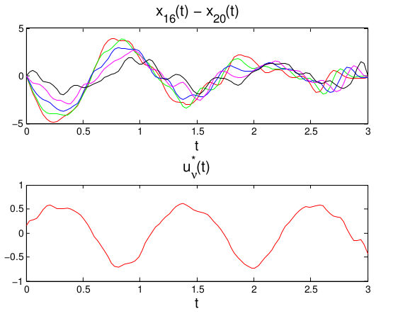
%% graphical part
t = linspace(0,T,nt+1);
figure;
subplot(2,1,1);
set(gcf,'DefaultAxesColorOrder',[1 0 0; 0 1 0; 0 0 1;1 0 1;0 0 0]) %red green blue yellow black
lc=N-4; uc=N; %choose the components of the system to be plotted, lc - the lowest comp. to be plotted, uc the most upper one
for i=lc:1:uc
plot(t,x(i,:));
hold all;
end
title(['x_{',num2str(lc),'}(t) - x_{',num2str(uc),'}(t)'],'Fontsize',15);
xlabel('t','Fontsize',14);
hold off;
subplot(2,1,2);
set(gcf,'DefaultAxesColorOrder',[1 0 0]) % red
plot(t,u);
title(['control for \nu=',num2str(nu_online)],'Fontsize',15);
xlabel('t','Fontsize',14);
if cc==1
%3d plot - wave eq.
figure;
y=0:1/(N/2+1):1;%discretisation of the domain [0,1]
sol=zeros(N/2+2,nt+1); %zero initiation
for i=2:N/2+1
sol(i,:)=x(i-1,:);
end
sol(N/2+2,:)=u;
mesh(y',t',sol','linewidth',2);
title(['v(t, x)'],'Fontsize',15);
xlabel('x','Fontname','Space variable','Fontsize',14,'Fontweight','b');
ylabel('t','Fontname','Time variable','Fontsize',14,'Fontweight','b');
end
if cc==2
%3d plot - heat eq.
figure;
y=0:1/(N+1):1;%discretisation of the domain [0,1]
sol=zeros(N+2,nt+1); %zero initiation
for i=2:N+1
sol(i,:)=x(i-1,:);
end
sol(N+2,:)=u;
mesh(y',t',sol','linewidth',2);
title(['v(t, x)'],'Fontsize',15);
xlabel('x','Fontname','Space variable','Fontsize',14,'Fontweight','b');
ylabel('t','Fontname','Time variable','Fontsize',14,'Fontweight','b');
end
Function adj_sol
%solves the adjoint problem p'=-A'p on [0,T] with datum p(T)=phi
%nt is the discretisation step of the time interval

function p=adj_sol(phi,T,nt,A)
p=zeros(size(phi,1),nt+1);
p(:,nt+1)=phi;
dt2=T/(2*nt);
R=speye(size(A))-dt2*A';
M=speye(size(A))+dt2*A';
for k=nt:-1:1
    p(:,k)=R\(M*p(:,k+1));
end
Function argmax
 %returns the (lowest) maximum position and the maximum value of the vector y
function[j,maks]=argmax(y)
j=1;
maks=y(1);
for i=2:1:length(y)
    if y(i)> maks;
        maks=y(i);
        j=i;
    end;
end
end
Function minFindAdjCG
%finding minimisator associated to the adjoint problem of the orig. control problem x'+Ax=Bu
% by using conj. gradient method
%the minimisator satisfies the system  Gq =rhs, where G- Gramiam, rhs=xf-  e(-TA)xi

function q=minFindAdjCG(xi,xf,T,nt,A,B,eps,qini)
%xi -initial data,
%xf - final target
%T-target time
%nt -# of discretisation steps in time interval
%eps -precision
%qini - initial guess of the solution

N=size(xi,1); %dimension of the system
x=sys_sol(xi,T,nt,-A, zeros(N,1), zeros(1,nt+1)); %solves the original problem in order to find find e(-TA)xi
rhs=xf-x(:,nt+1);
nb=norm(rhs);
if nb==0, nb=1; end

%Finding G*qini
q=qini;
p_q=adj_sol(q,T,nt,-A); %p- solution of the adjoint problem
u_q=B'*p_q;
x_q=sys_sol(zeros(N,1),T,nt,-A, B, u_q); %x- solution of the original problem
Gq=x_q(:,nt+1);

M_inv=eye(N);%preconditioning matrix M_inv, symmetric, posit. def.
r=rhs-Gq; %residual r_0
z=M_inv*r; %if no preconditioning, z =r
h=z; % h stands for the next direction of the method
z_=z;
r_=r;
ng_=r'*r; %error norm
k=0;
nitermax=min(1000,size(xi,1)^2);
while k<nitermax && ng_>eps^2,
    %Finding G*h
    p_h=adj_sol(h,T,nt,-A);
    u_h=B'*p_h;
    x_h=sys_sol(zeros(N,1),T,nt,-A, B, u_h);
    Gh=x_h(:,nt+1);
    alpha=(r'*z)/(h'*Gh);
    q=q+alpha*h; %finding (k+1). aproximation
    r=r-alpha*Gh;  %next residual r_(k+1)
    z=M_inv*r;
    beta=z'*r/(z_'*r_);
    h=z+beta*h; % finding the next direction of the method
    ng=r'*r;
    ng_=ng;
    z_=z; %store the residual for the next iteration
    r_=r;
    k=k+1;
end

if 1%check the error Gq-rhs
    p_q=adj_sol(q,T,nt,-A);
    u_q=B'*p_q;
    x_q=sys_sol(zeros(N,1),T,nt,-A, B, u_q);
    Gq=x_q(:,nt+1);
    err=norm(Gq-rhs); %it corresponds to deviation of the solution at time T from the target: |x(T)-xf|
    fprintf(['minFindAdj:: number of iteration reached:', num2str(k),'\n error: ', num2str(err),'\n']);
end
if k>=nitermax,
    fprintf(['minFindAdj:: maximal number of iteration reached, error: \n',num2str(ng)]);
end
end
Function projection
%provides the orthogonal projection of a vector v to the space spanned by
%columns of matrix B

function  [y]=projection(v,B)
g=orth(B);  %gram-schmidt orthogonalisation
m=size(g,1);
n=size(g,2);

y=zeros(m,1);
%calculation of the projection
for j=1:1:n
    y=y+dot(v,g(:,j))*g(:,j);
end

end
Function sys_sol
%solves the system x'=Ax+bu on [0,T] with datum x0
%nt is the discretisation step of the time interval
function x=sys_sol(x0,T,nt,A,b,u)
x=zeros(size(x0,1),nt+1);
x(:,1)=x0;
dt2=T/(2*nt);
R=speye(size(A))-dt2*A;
M=speye(size(A))+dt2*A;
B=dt2*b;
for k=1:nt,
    x(:,k+1)=R\(M*x(:,k)+B*(u(k)+u(k+1)));
end