
Spain. 24.02.2021
Author: Sergi Andreu
Opening the black box of Deep Learning
Its impact in modern technologies is huge. However, there is not a clear high-level description of what these algorithms are actually doing.
In this sense, Deep Learning models are sometimes referred to as “black box models”; that is, we can characterize the models by its inputs and outputs, but with any knowledge of its internal workings.
The aim is then to open the black box of Deep Learning, and try to gain an intuition of what are these models doing. One of the most successful mathematical theories in recent years has been connecting Deep Learning with Dynamical Systems.
The aim of this post is to introduce to some of those exciting ideas.
Data and classification
Supervised Learning
Deep Learning essentially wants to solve the problem of Supervised Learning. That is, we want to learn a function that maps an input to an output, based on examples of input-output pairs.
A classical Deep Learning problem would be the following: we have some pictures of cats and dogs, and want to make an algorithm that learns when the input image shows a dog and when it shows a cat. Note that we could give the algorithm pictures that it has not previously seen, and the algorithm should label the pictures correctly.
A formal description of our problem is the following.
Consider a dataset \mathcal{D} consisting on S distinct points \{x_i\}_{i=1}^{S}, each of them with a corresponding value y_i such that
\mathcal{D} = \{(x_i , y_i)\}_{i=1}^Swe expect that the labels y_i are a function of x, such that
y_i = \mathcal{F} (x_i) + \epsilon _i \quad \forall i \in \{1, ... S\}
where \epsilon _i is included so as to consider, in principle, noisy data.
The aim of supervised learning is to recover the function \mathcal{F}(\cdot) such that not only fits well in the database \mathcal{D} but also generalises to previously unseen data.
That is, it is inferred the existence of
\tilde{\mathcal{D}} = \{ (\tilde{x}_i , \tilde{y}_i) \}_{i=1}^{\infty}
where
\tilde{y}_i \approx \mathcal{F}(\tilde{x}_i) \quad \forall i
being \mathcal{F} (\cdot) the desired previous application, and \mathcal{D} \subset \tilde{\mathcal{D}}.
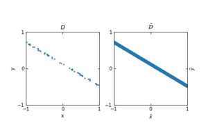
The figure in the left represents a finite set of points in (x,y), where x represents the input and y the output. The figure on the right is the expected distribution from which we are sampling the input-output examples. The whole distribution can be understood by \tilde{\mathcal{D}}.
A well-known dataset in which to use Deep Learning algorithm is the CIFAR-10 dataset.
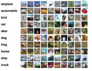
Scheme of the CIFAR-10 dataset
In this case, the input images consist on a value in [0,1] for each pixel and Red / Green / Blue color. Since the resolution is 32 \times 32 pixels, the input space would be [0,1]^d with d=32 \times 32 \times 3 = 3072. Each image has a correspondent label (airplane, automobile, …).
The dataset is then given by \{ x_j, y_j = f^*(x_j)\} where the inputs x_j \in [0,1]^{3072}, and the labelling function acts as f^* : [0,1]^{3072} \to \{ \text{airplane, automobile, ... } \}.
We want that f^*( \text{each image} ) = \text{correct label of that image}.
Note that the function f^* we are talking about is not the same as the function \mathcal{F} that we used when defining the notion of dataset. This is because the function f^* is the application that connects the images with their given labels, whereas the function \mathcal{F} is the function that connects any feasible input image with its *true* label. We have access to $f^*$, but not \mathcal{F}.
Noisy vs. noisless data
What are the true labels of a dataset? We have no a priori idea. What is the mathematical definition of “pictures of airplanes”? Our best guess is to learn the definition by seing examples.
However, those examples may be mistakenly labelled, since the datasets are in general noisy. What does a noisy dataset mean?
– We refer to noisy data when the samples in our dataset \tilde{\mathcal{D}} actually comes from a random vector (\mathbf{x}, \mathbf{y}) with a non-deterministic joint distribution, such that it is not possible to find a function \mathcal{F} such that \mathcal{F}(\mathbf{x}) = \mathbf{y}.
The aim of *supervised learning*, in this case, would be to find a function such that \mathcal{F}(\mathbf{x}) \approx \mathbf{y}. For example, \mathcal{F}(\tilde{x}_i) = \tilde{y}_i for almost every sample i.
– In the case of noisless data (which does not happen in most practical situations, but it makes things far simpler) then it is possible to find a function \mathcal{F} such that \mathcal{F}(\tilde{x}_i) = \tilde{y}_i \; \forall i, or equivalently \mathcal{F}(\mathbf{x}) = \mathbf{y}.
Note that, given that the probability of a collision (of having two different data-points such that x_i = x_j for i \neq j) is practically 0, it is in principle possible to find a function \mathcal{F} such that \mathcal{F}(x_i)=y_i for all of our samples i, even in the noisy case (for example, we may use interpolation).
However, the aim of supervised learning is to be able to generalise well to previously unseen data, \tilde{\mathcal{D}}, and so interpolation is not effective, and may not be well-defined, since the same input x_i can be labelled differently, due to noise.
Representation of the optimal function \mathcal{F} as the number of samples increases, in the case of noisy data. Note that the function “stabilizes” at a certain point, and thus it is expected to behave properly in the limit of infinitely many samples.
Representation of the optimal function \mathcal{F} as the number of samples increases, in the case of noisless data. In this case the function could have been obtained by interpolation, and would stabilize fast
Binary classification
In most cases, the data points x_i are in \mathbb{R}^{n}. In general, we may restrict to a subspace of feasible images X \in \mathbb{R}^{n}.
So as to ease the training of the models, the inputs are usually normalized, and it is considered X = [-1,+1]^{n}, with n the input dimension.
There are different supervised learning problems depending on the space Y of the labels.
If Y is discrete, such that Y = \{ 0, ... , L-1\}, then we are dealing with the problem of classification. In the case of CIFAR-10 we have 10 classes, and so L=10.
If L=2, then it is a binary classification problem, such as in the case of classifying images of cats and dogs (in this case, dog may be represented by “0” and cat by “1”).
In the particular setting of binary classification, the aim is to find a function \mathcal{F} (x) such that it returns 0 whenever the corresponding data point x is of class 0, and 1 conversely.
Data, subspaces and manifolds
Consider M^0 the subset of X such that F( \tilde{x} _i) =0 for all the points \tilde{x}_i in M^0. And consider M^1 such that \, F(\tilde{x}_i)=1 for all the points in M^1.
It is useful to consider d(M^0 , M^1) > \delta. That is, we want the subspace of images of cats and the subspace of images of dogs to have a nonzero distance in the input space. This makes sense physically, since we do not expect the pictures of dogs and cats to overlap.
An interesting hypothesis is to consider that M^0 and M^1 are indeed manifolds in a low-dimensional space. This is called the manifold hypothesis.
That is, out of the whole input space of all possible images, only a low-dimensional subspace of those would correspond to the images of cats, and one could go from one picture of a cat to any other picture of a cat by a path in which all the point are also pictures of cats. This has been widely hypothesized in many datasets, and there are some experimental results in that direction [9].
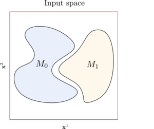
Example of the input space in a binary classification setting. The axis \mathbf{x}^1 and \mathbf{x}^2 represent the components of the vectors x the input space (we are considering [0,1]^2). The points in the subspace M_0 are labelled as 0, and the points in M_1 as 1. The points that are not in M_0 or M_1 do not have a well-defined label.
// This post continues on post: Deep Learning & Paradigms
References
[1] J. Behrmann, W. Grathwohl, R. T. Q. Chen, D. Duvenaud, J. Jacobsen. Invertible Residual Networks (2018) [2] Weinan E, Jiequn Han, Qianxiao Li. A Mean-Field Optimal Control Formulation of Deep Learning. Vol. 6. Research in the Mathematical Sciences (2018) [4] B. Hanin. Which Neural Net Architectures Give Rise to Exploding and Vanishing Gradients? (2018) [5] C. Olah. Neural Networks, Manifolds and Topology [blog post] [6] G. Naitzat, A. Zhitnikov, L-H. Lim. Topology of Deep Neural Networks (2020) [7] Q. Li, T. Lin, Z. Shen. Deep Learning via Dynamical Systems: An Approximation Perspective (2019) [8] B. Geshkovski. The interplay of control and deep learning [blog post] [9] C. Fefferman, S. Mitter, H. Narayanan. Testing the manifold hypothesis [pdf] [10] R. T. Q. Chen, Y. Rubanova, J. Bettencourt, D. Duvenaud. Neural Ordinary Differential Equations (2018) [11] G. Cybenko. Approximation by Superpositions of a Sigmoidal Function [pdf] [12] Weinan E, Chao Ma, S. Wojtowytsch, L. Wu. Towards a Mathematical Understanding of Neural Network-Based Machine Learning_ what we know and what we don’t [14] Introduction to TensorFlow [tutorial] [15] C. Esteve, B. Geshkovski, D. Pighin, E. Zuazua. Large-time asymptotics in deep learning [16] Turnpike in a Nutshell [Collection of talks]More about: ERC DyCon project
|| See more posts at DyCon blog