Swinging up the double pendulum on a cart

Spain. 24.01.2022
Author: Arnaud Rippol

Introduction

Pendulums are systems often used in Control Theory or Reinforcement Learning as benchmarks examples to prove the efficiency of some methods or algorithms. The first basic problem one may want to solve is the stabilization problem: starting from the upward, unstable position, a small control is applied to maintain the pendulum in equilibrium. The swinging-up problem is more complex: this time, the pendulum starts from the bottom position, and we want to apply a control to reach the upward position and to stay there.

Many kinds of pendulums exist. The most simple is a rod with one extremity kept fixed, and with one weight on the other side: one could apply a torque to move the system in oscillations from left to right. In itself, this system is already interesting because of its non-linearity, which means that many techniques cannot perform well far from the two balanced positions and are therefore unable to perform swing-ups.

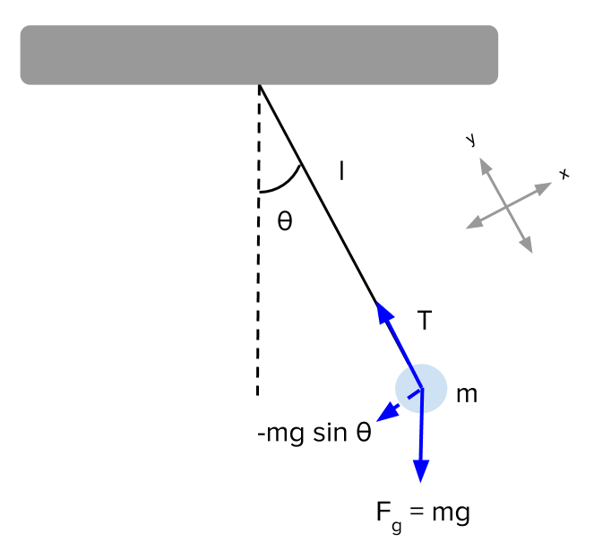
Figure 1 – Pendulum

The equation of the dynamics is

\frac{\partial^2\theta}{\partial t^2} = - \frac{g}{l} \sin\theta (1.1)
in which the non-linearity appears in \sin\theta.

From this system, we can extend to multiple pendulums: several identical systems are linked together, the “fixed” extremity of one being the end of another one. These systems add more complexity to our swinging-up problem due to their chaotic aspect: as soon as we have at least a double pendulum, the whole system becomes chaotic, meaning that a small change in the initial conditions leads to a great difference in the dynamics.
However, applying torques is a very direct control of the system, with a direct impact on the angles, which makes the previous problems quite easy to solve. The system investigated here is a double pendulum on a cart.

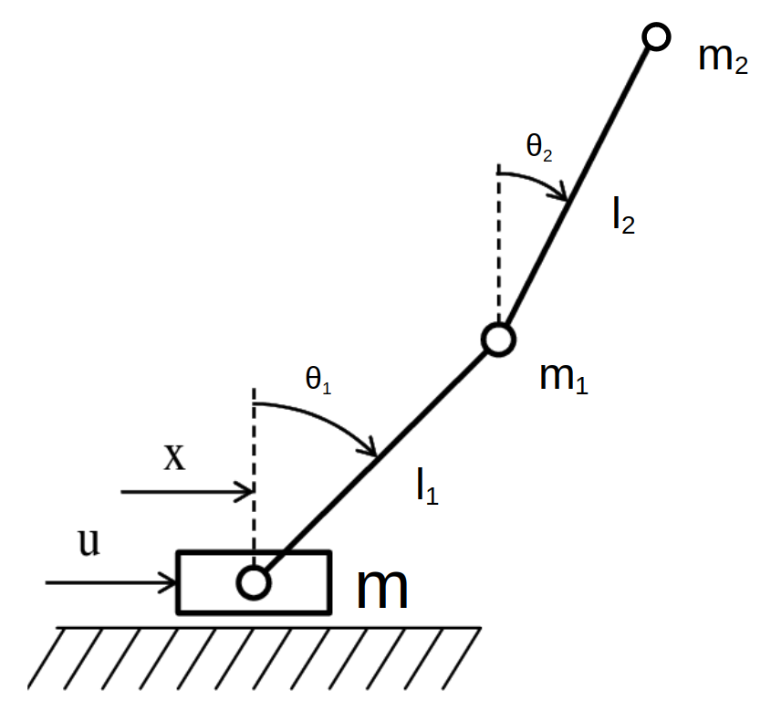
Figure 2 – The double pendulum on a cart

The purpose of this study is to compare different ways to control complex system and to compare their efficiency. The interests of the double pendulum on a cart is that it is a complex non-linear, chaotic system, which makes it a “difficult” problem to solve. On the other hand, it has a small number of degrees of freedom, and a control in one dimension only, which makes it easier to compute, especially when investigating Reinforcement Learning methods.

As for the notation, we will call the state vector and the control at time t respectively y(t) and u(t). y(t) is a vector with 6 dimensions: y = (x, \theta_1, \theta_2, v, \omega_1, \omega_2) where x is the position along the horizontal axis, \theta_1 and \theta_1 are the angles between the first/second rod and the vertical axis, and v, \omega_1 and \omega_2 are the derivatives of x, \theta_1, \theta_2, i.e. the horizontal speed and the angular speeds of both rods.
The control u is the horizontal acceleration given to the cart.

We therefore have y(t)\in\mathbb R^6 and u(t)\in\mathbb R.

We introduce the dynamical function f that takes the current state and a control and gives the derivative of the state:
f(y(t), u(t)) = \dot{y}(t).

We can also define the step function
F(y(t), u(t)) = \int_t^{t+\Delta t} f(y(t), u(t))

that given a state and a control returns the next state, \Delta t later.

Optimal Control

Optimal control is a field in mathematics that tries to find a control to minimize a certain loss function. For y(t) the state vector and u(t) the control vector at time t, we try to minimize the following function:

J(\mathbf{u}) = \Phi(y(T), u(T), T) + \int_{t_0}^T \Psi(y(t), u(t), t) \mathrm{d}t

In this work, since we are focusing on a discrete problem, the shape of the loss function is actually:

J(\mathbf{u}) = \Phi(y(T), u(T), T) + \sum_{i = 0}^N \Psi(y(i\cdot\Delta t), u(i\cdot\Delta t), i\cdot\Delta t)

where N is the number of steps in the simulations and \Delta t is the interval of time between 2 steps.

In other words, we want to optimize \textbf{u} = (u_1,\dots, u_N) to minimize J with the dynamical constrain:

\begin{cases} \displaystyle\min_{\textbf{u}\in U} J(\textbf{u}) \\ s.t. \forall i=0,\dots,N-1, y((i+1)\Delta t) = F(y(i \Delta t), u_i) \end{cases}

where F is the step function defined in (1).

One difficulty with this problem comes from the shape of the dynamical function f which is not linear. If we had y'(t) = A y(t) + B u(t) with A \in \mathbb{R}^{6×6} ,B \in \mathbb{R}^{6×1} two constant matrices, other approaches could be used, for instance Linear–quadratic regulator which solve our optimal control in a closed-form way, with a feedback loop. Since it is not the case, we are using solvers to help us getting an optimal trajectory.

Many forms of software exist to solve problems with the form of 1. In this study, we used IPOPT (Interior Point OPTimizer), which is renown and widely used in the dynamical control field.

To obtain a control with IPOPT, we need to specify the loss function that we want to use. In our case, we want to reach a specific position, y_f = (0,0,0,0,0,0), so we choose the function \Phi in 2 to be

\Phi(y(T), u(T), T) = \alpha ||y(T)||^2

We also want to reach this position as directly as possible (i.e. without a lot of movement on the track) and with a limited control, so we choose

\Psi(y(t), u(t), t) = \beta ||y(t)||^2 + \gamma u(t)^2

We also need to choose U, the space in which we can choose the control. Since we want the control to be plausible, it cannot take too large values, so we have U = [−u_{max},u_{max}]^N. Based on values seen on real simulations, we selected u_{max} = 10m\cdot s^{-2}.

However, we still need to figure out what are the parameters \alpha, \beta, \gamma in the definitions of \Psi and \Phi. For this, the only solution was by heuristic, checking whether or not the solution of the solver reaches the target. These are hyper-parameters that require expert knowledge and prevent this method to be completely transposable to another system. In this study, the parameters used were \alpha = 1000, \beta = 1, \gamma = 0.05.

Furthermore, after some iterations, the actual trajectory of the pendulum of our implementation diverges from the nominal one due to the chaotic aspect of the system, so the upward position is missed and the pendulum does not reach its equilibrium.

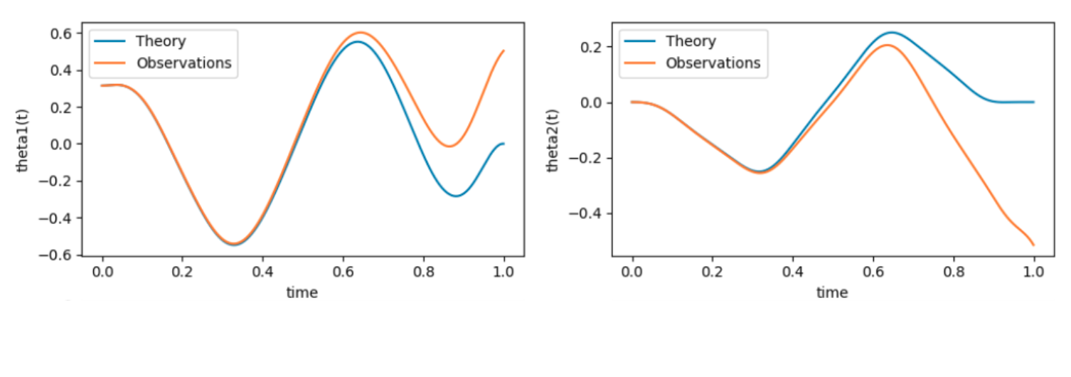
Figure 3 – A consequence of the chaotic aspect of the pendulum

Therefore, the feedforward trajectory alone is not enough and we need to find a way to maintain the trajectory near the nominal one. We will implement a feedback strategy to solve this problem.

We will note y^*(t) the computed optimal trajectory, y(t) the actual trajectory simulated, and \Delta y(t) = y(t) - y^*(t) the difference between the two trajectories.

The goal of the feedback is to keep \Delta y as close as possible to (0,\dots,0) by adding an extra control \Delta u at each point. If this difference is maintained quite small, we can linearize the control equation at each moment in time to get

\Delta y'(t) = A(t) \Delta y(t) + b(t) \Delta u(t) with A(t) = \left. \frac{\partial f}{\partial y} \right |_{y^*(t), u^*(t)} and b(t) = \left. \frac{\partial f}{\partial u} \right |_{y^*(t), u^*(t)}.

At each step, we want to minimize the gap between nominal and real trajectory. To do so, we minimize the following loss:

L_i = \Delta y_i^T Q \Delta y_i + \Delta u_i R \Delta u_i

with Q = diag(1, 1, 1000, 1, 1, 200) and R=1.

We can then solve the systems composed of the two previous equations at each step, which we do like a real linear quadratic one: we compute P the solution of the Riccati equation:

\left\{ \begin{array}{cc}. P'& =&-PA(t) - A(t)^TP +Pb(t)R^{-1}b(t)^TP - Q \\ P(T)&=&0 \end{array} \right.

Then we obtain the feedback gain as k(t) = R^{-1} b(t) P(t) and we obtain the control with feedback as follows
u(t) = u^*(t) - k(t)^T\Delta y(t)

For our parameters (N = 100 points and T = 5s), the time to get the final control is about 16 seconds. However, in order to get a good trajectory, the exact weights are needed and an “expert knowledge” is required. Therefore, we tried to obtain the same results using methods from another field: Reinforcement Learning.

Reinforcement Learning

**Reinforcement Learning** (RL) is a way to tackle problems that is quite different from the other data-driven techniques. There is an agent evolving in an environment, taking actions depending on its state, and receiving rewards based on its action and the environment, following a policy and aiming to maximize its total reward. We have the following usual notations:

– \mathcal{S} the state space,

– \mathcal A the action space,

– \mathbb{P}(s'|s,a) the transition function that takes the current state s and an action a and gives a probability distribution of the next state s',

– \mathcal{R}(s,a,s') the reward function,

– \pi : \mathcal S \rightarrow \mathcal A a policy.

In our context, \mathcal S is the set of the possible value taken by our system, which is \mathbb{R}^6 ; \mathcal A is the space of the control, which is \mathbb{R} ; P is actually a deterministic function, which is F defined in (1). Our goal is to find a way to use \mathcal{R} and \pi so that we can reach our target, which is swinging-up the double pendulum on a cart.
A classical approach in Reinforcement learning introduces the following elements:

– the Return at time t: R_t = \sum_{i=0}^{T-t-1} \gamma^i r_{i+t+1} with \gamma \in (0, 1] a discount factor.

– the Action-Value function: Q^{\pi}(s, a) = \mathbb E[R_t|s_t = s, a_t = a]

An example of policy would be the Greedy policy, which consists in:
\pi(s) = \underset{a\in\mathcal A}{\arg\!\max} \:Q(s_t, a)

The problem is then to find an approximation for the value of the function Q, which can be very difficult and long, and is at the core of Q-learning, a classical reinforcement learning algorithm.

The problem at stake in Reinforcement Learning is much harder that the one in optimal control. The purpose here is not to learn a single trajectory, but to compute a whole function, the policy \pi. Therefore, the computational time is expected to be longer, but on the other hand, ending up with a function is a great advantage. Indeed, we are able to reuse it as much as wanted, with different initial conditions, unlike the control obtained with the previous techniques.

Among all the reinforcement learning algorithm, only one is able to solve our problem and swing-up the double pendulum on a cart: PILCO (Probabilistic Inference for Learning COntrol). This algorithm was a breakthrough for its speed and performance on complex system, including ours.

It is a model-based algorithm: to learn the policy, the algorithm also uses a model to learn the dynamic function. In the case of PILCO, we consider the function f: x_t \mapsto y_{t+1} to be a **Gaussian Process**, with x_t := (y_t , u_t) \in \mathbb R^7 :

\begin{cases} \forall (x_1, \dots, x_n), (f(x_1), \dots, f(x_n)) &\text{ is a Gaussian vector},\\ m(x) := \mathbb{E}[f(x)] &\text{ is the mean function},\\ k(x, x') := \mathbb{E}[(f(x)-m(x))(f(x')-m(x'))] &\text{ is the covariate function, or kernel} \end{cases}

In PILCO, we assume that the kernel is Squared Exponential:
k(x, x') = \alpha^2 \exp\left(-\frac{1}{2}(x-x')^TS(x-x')\right) with \alpha and S to be learned.

The randomness of the function embeds the uncertainty of the dynamics at the beginning of the learning. As the algorithm is running, the uncertainty diminishes, up to a point at which the swinging-up can be performed. At each step, we use the best policy given the current data available, and we record the obtained trajectory to improve our policy: it is a Bayesian approach.

We use the following shape for the policy of our model:

\pi(y, \theta) = \sum_{i=0}^M \omega_i\Phi_i(y), \text{ where } \Phi_i(y) = \exp\left(-\frac{1}{2}(y-\mu_i)^T\Lambda(y-\mu_i)\right)

with \theta = (\Lambda, \omega_1, \mu_1, \dots, \omega_M, \mu_M) is the parameter of the policy, and M a parameter chosen before running the algorithm. Note that this shape is used for all application of PILCO and is therefore not an expert knowledge.

Instead of a reward function that we want to maximize, we talk about a cost function that we minimize. In the case of PILCO, it has the following shape:

\begin{cases} &\text{Cost of one state: } & c(y) = 1 - \exp(-||y||^2/\sigma_c^2) \\ &\text{Cost of the policy: } & J(\theta) = \sum_{t=1}^N\mathbb{E}[c(y_t)] \end{cases}

where distribution of probability for y_t at each step is computed recursively: y_{t+1} \sim f(y_t, \pi(y_t, \theta)).

At first, we have no information on the behavior of f. To gain information, a first random rollout is done: actions

(u_t)_0≤t<N ∈ U^N

are chosen randomly and we record the data f(y_t, u_t)=y_{t+1}.

Thanks to these new data points, we can reduce the space in which f can be:

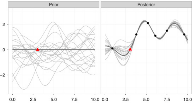
Figure 4 – The learning of the Gaussian Process. The x-axis is a 1-dimension representation of (y_t,u_t) and the y-axis is a 1 dimension representation of y_{t+1}.

We can therefore develop the following algorithm:

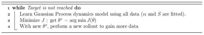
Each step requires a lot of math but everything can be done analytically, including the gradient of J which can be written down and used for the minimization process.
For this problem, we have one hyper-parameter that needs to be chosen before launching the learning: M, the number of components for the policy. If this number is too big, the learning will take too much time; if it is too low, there isn’t enough complexity to capture the movement of the system and the goal will never be reached.

PICLO is a state-of-the-art algorithm because it manages to solve new problems with reinforcement learning, and because it does so with very little interaction with the system. For the double pendulum problem, less than 30 iterations of 5 seconds are needed to swing-up and balance the double pendulum on a cart. However, this efficiency must not be taken for a quick way to solve this problem. Indeed, it takes several hours and a lot of memory to perform the learning. On a computer (8Gb of RAM), we cannot perform more than the 5 first iterations without running out of memory, and it takes about 9 hours.

Mixing Reinforcement Learning and Optimal Control

To solve our problem, which is to swing-up the double pendulum on a cart, we have tackled two different approaches so far. The first one comes from the optimal control theory: it is quick to compute, but not reusable with different initial conditions since we only get one trajectory. The second solution is reinforcement learning, which gives us a final function that we hope to be reusable, but is very long to compute. One can wonder if we can mix these two aspects to get a better algorithm, which returns the function of reinforcement learning, but does not need as much computational time as PILCO alone, which is very long.

Instead of starting from scratch with a random rollout, we first compute a winning trajectory, which we can use to train the Gaussian process that models the dynamical function. The objective is to eliminate uncertainty on a part of the space that we know to have a very low cost, since it solves our problem. However, a region of high uncertainty means also a high possible outcome, even if it’s not the case. Therefore, the algorithm still needs to eliminate the potentially good outcomes and must make several tries before exploring the area near the pre-computed trajectory. Since the stabilization still takes about 10 steps in the literature, though it is a much more easier task than the swing-up, we decided to add some trajectory computed with starting points near the upper equilibrium, so as to speed up this process and hopefully balance the pendulum quickly after it reaches the upward position.

Unfortunately, as explained before, complete results cannot be presented due to the high computational time, but the 13 first iterations of the process were calculated.
However, even after 13 iterations, it seems the algorithm hasn’t learn anything yet. The loss function stays above 99 for each iterations, the best values being 0 and the worst 100. This result is even more surprising when comparing with the literature: since the complete swinging-up occur at about 15 iterations, we could expect the loss to start dropping several iterations before that.
Several reasons could explain this phenomenon. The first could be that the loss actually starts dropping in the following iterations, which would mean that the addition of previous knowledge the way we did has roughly no impact on PILCO, and that the poor performance is simply due to the random aspects in the algorithm (a different seem can lead to different results). The second explanation would be a software problem in the PICLO algorithm itself. Since our version of the unmodified algorithm has been tested successfully on another problem, it means that the problem would come from the modification we performed: the choice in the starting point for the optimization process.