PDF version… | Download Code… | Related Paper…
The problems considered
We obtain a finite element (FE) scheme for the numerical approximation of the solution to the following non-local Poisson equation
\begin{align}
\begin{cases}
\fl{s}{u} = f, \quad & x\in(-L,L)
\\
u\equiv 0, & x\in\RR\setminus(-L,L).
\end{cases}
\end{align}
In (1), $f$ is a given function and, for all $s\in(0,1)$, $\fl{s}{}$ denotes the one-dimensional fractional Laplace operator, which is defined as the following singular integral
\begin{align}\label{fl}
\fl{s}{u}(x) = \ccs\,P.V.\,\int_{\RR}\frac{u(x)-u(y)}{|x-y|^{1+2s}}\,dy.
\end{align}
Here, $\ccs$ is an explicit normalization constant.
The main novelty of this work relies on the fact that, since we are dealing with a one-dimensional problem, each entry of the stiffness matrix can be computed explicitly, without requiring numerical integration, which is instead needed for the multidimensional case (see [1]). This has the great advantage of reducing the computational cost and allows to be used on more general applications.
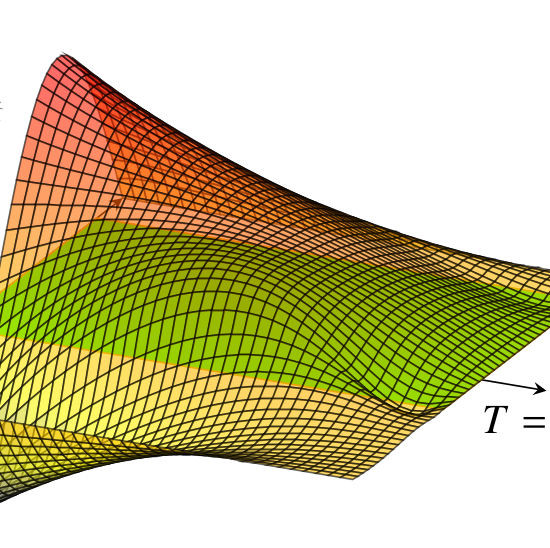
A natural example is given by the numerical resolution of the following control problem: given any $T>0$, find a control function $g\in L^2((-1,1)\times(0,T))$ such that the corresponding solution to the parabolic problem
\begin{align}
\begin{cases}
z_t + \fl{s}{z} = g\mathbf{1}_{\omega},\quad & (x,t)\in (-1,1)\times(0,T)
\\
z=0, & (x,t)\in[\,\RR\setminus (-1,1)\,]\times(0,T)
\\
z(x,0)=z_0(x), & x\in (-1,1)
\end{cases}
\end{align}
satisfies $z(x,T)=0$.
The approach emploied for solving this control problem is based on the penalized Hilbert Uniqueness Method ([2]).
Preliminary results
Variational formulation of the elliptic problem
Find $u\in H^s_0(-L,L)$ such that
\begin{align*}
\frac{\ccs}{2} \int_{\RR}\int_{\RR}\frac{(u(x)-u(y))(v(x)-v(y))}{|x-y|^{1+2s}}\,dxdy = \int_{-L}^L fv\,dx,
\end{align*}
for all $v\in H_0^s(-L,L)$. Here, $H^s_0(-L,L)$ denotes the space
\begin{align*}
H^s_0(-L,L) :=\Big\{\, u\in H^s(\RR)\,:\,u=0 \textrm{ in } \RR\setminus(-L,L)\,\Big\},
\end{align*}
while $H^s(\RR)$ is the classical fractional Sobolev space of order s. Since the bilinear form a is continuous and coercive, Lax-Milgram Theorem immediately implies that, if $f\in H^{-s}(-L,L)$, the dual space of $H^s_0(-L,L)$, then (1) admits a unique weak solution $u\in H_0^s(-L,L)$.
Parabolic problem
Definition 1. System (3) is said to be null-controllable at time $T$ if, for any $z_0\in L^2(-1,1)$, there exists $g\in L^2((-1,1)\times(0,T))$ such that the corresponding solution $z$ satisfies
\begin{align*}
z(x,T)=0.
\end{align*}
Definition 2. System (3) is said to be approximately controllable at time $T$ if, for any $z_0,z_T\in L^2(-1,1)$ and any $\delta>0$, there exists $g\in L^2((-1,1)\times(0,T))$ such that the corresponding solution $z$ satisfies
\begin{align*}
[+preamble]
\renewcommand{\norm}[2]{{\left\|#1\right\|}_{#2}}
[/preamble]
\norm{z(x,T)-z_T}{L^2(-1,1)}<\delta.
\end{align*}
There are few results in the literature on the null-controllability of the fractional heat equation, and they all deal with the spectral definition of the fractional Laplace operator, which is introduced, e.g., in [3],[4]. In this framework, it is known that the fractional heat equation is null-controllable, provided that $s>1/2$. For $s\leq 1/2$, instead, null controllability does not hold, not even for $T$ large.
However, also for the parabolic equation involving the integral fractional Laplacian (2), at least in the one space dimension, these properties are easily achievable. In more detail, we prove the following.
Proposition 1. For all $z_0\in L^2(-1,1)$ the parabolic problem (3) is null-controllable with a control function $g\in L^2(\omega\times(0,T))$ if and only if $s>1/2$.
Even if for $s\leq 1/2$ null controllability for (3) fails, we still have the following result of approximate controllability.
Proposition 2. Let $s\in(0,1)$. For all $z_0\in L^2(-1,1)$, there exists a control function $g\in L^2(\omega\times(0,T))$ such that the unique solution $z$ to the parabolic problem (3) is approximately controllable.
Development of the numerical scheme
Finite element approximation of the elliptic problem
Let us introduce a partition of the interval $(-L,L)$ as follows:
\begin{align*}
-L = x_0<x_1<\ldots <x_i<x_{i+1}<\ldots<x_{N+1}=L\,, \end{align*} with $x_{i+1}=x_i+h$, $i=0,\ldots N$, $h>0$. Having defined $K_i:=[x_i,x_{i+1}]$ we consider the discrete space
\begin{align*}
V_h :=\Big\{v\in H_0^s(-L,L)\,\big|\, \left. v\,\right|_{K_i}\in \mathcal{P}^1\Big\},
\end{align*}
where $\mathcal{P}^1$ is the space of the continuous and piece-wise linear functions. If we indicate with $\big\{\phi_i\big\}_{i=1}^N$ the classical basis of $V_h$ in which each $\phi_i$ is the tent function with $supp(\phi_i)=(x_{i-1},x_{i+1})$ and verifying $\phi_i(x_j)=\delta_{i,j}$, at the end we are reduced to solve the linear system
\begin{align*}
\mathcal A_h u=F,
\end{align*}
where the stiffness matrix $\mathcal A_h\in \RR^{N\times N}$ has components
\begin{align}\label{stiffness_nc}
a_{i,j}=\frac{\ccs}{2} \int_{\RR}\int_{\RR}\frac{(\phi_i(x)-\phi_i(y))(\phi_j(x)-\phi_j(y))}{|x-y|^{1+2s}}\,dxdy, \;\;\; i,j = 1,\ldots,N,
\end{align}
while the vector $F\in\RR^N$ is given by $F=(F_1,\ldots,F_N)$ with
\begin{align*}
F_i = \langle f,\phi_i\rangle = \int_{-L}^L f\phi_i\,dx,\;\;\; i=1,\ldots,N.
\end{align*}
The construction of the stiffness matrix $\mathcal A_h$ is done in three steps, since its elements can be computed differentiating among three well defined regions: the upper triangle, corresponding to indices $j\geq i+2$, the upper diagonal corresponding to $j=i+1$, and the diagonal corresponding to $j=i$. In each of these regions, the intersections among the support of the basis functions are different, thus generating different values of the bilinear form.
After several computations, we obtain the following expressions for the elements of the stiffness matrix $\mathcal{A}_h$: for $s\neq 1/2$
\begin{align*}
a_{i,j} = -h^{1-2s} \begin{cases}
\displaystyle \,\frac{4(k+1)^{3-2s} + 4(k-1)^{3-2s}-6k^{3-2s}-(k+2)^{3-2s}-(k-2)^{3-2s}}{2s(1-2s)(1-s)(3-2s)}, & \displaystyle k=j-i,\,k\geq 2
\\
\\
\displaystyle\frac{3^{3-2s}-2^{5-2s}+7}{2s(1-2s)(1-s)(3-2s)}, & \displaystyle j=i+1
\\
\\
\displaystyle\frac{2^{3-2s}-4}{s(1-2s)(1-s)(3-2s)}, & \displaystyle j=i.
\end{cases}
\end{align*}
For $s=1/2$, instead, we have
\begin{align*}
a_{i,j} = \begin{cases}
-4(j-i+1)^2\log(j-i+1)-4(j-i-1)^2\log(j-i-1)
\\
\;\;\;+6(j-i)^2\log(j-i)+(j-i+2)^2\log(j-i+2)+(j-i-2)^2\log(j-i-2), & \displaystyle j> i+2
\\
\\
56\ln(2)-36\ln(3), & \displaystyle j= i+2.
\\
\\
\displaystyle 9\ln 3-16\ln 2, & \displaystyle j=i+1
\\
\\
\displaystyle 8\ln 2, & \displaystyle j=i.
\end{cases}
\end{align*}
Control problem for the fractional heat equation
We employ the so called penalised Hilbert Uniqueness Method (HUM) that deals with the resolution of the following minimization problem: find
\begin{align}\label{min_je}
\varphi^T_\varepsilon=\min_{\varphi\in L^2(-1,1)} J_\varepsilon (\varphi^T)
\end{align}
where
\begin{align}\label{penalized_fun}
[+preamble]
\renewcommand{\norm}[2]{{\left\|#1\right\|}_{#2}}
[/preamble]
J_\varepsilon(\phi^T):=\frac{1}{2}\int_0^T\int_{\omega}|\varphi|^2\,dxdt + \frac{\varepsilon}{2}\norm{\varphi^T}{L^2(-1,1)}^2 + \int_{\Omega} z_0\varphi(0)\,dx,
\end{align}
where $\varphi$ is the solution to the adjoint problem
\begin{align*}
\begin{cases}
-\varphi_t+\fl{s}{\varphi}=0, & (x,t)\in (-1,1)\times(0,T)
\\
\varphi = 0, & (x,t)\in\big[\RR\setminus(-1,1)\big]\times(0,T)
\\
\varphi(x,T)=\varphi^T(x), & x\in (-1,1).
\end{cases}
\end{align*}
Then, the approximate and null controllability properties of the system, for a given initial datum $z_0$, can be expressed in terms of the behavior of the penalized HUM approach. In particular, according to [2,Theorem 1.7] we have:
-
- The equation is approximately controllable at time $T$ from the initial datum $z_0$ if and only if
\begin{align*}
\varphi_\varepsilon^T\rightarrow 0,\;\;\;\textrm{ as }\;\varepsilon\to 0.
\end{align*}
-
- The equation is null-controllable at time $T$ from the initial datum $z_0$ if and only if
\begin{align*}
M_{z_0}^2:=2\sup_{\varepsilon>0}\left( \inf_{L^2(0,T;L^2(\omega))}J_\varepsilon\right)<+\infty.
\end{align*}
In this case, we have
\begin{align*}
[+preamble]
\renewcommand{\norm}[2]{{\left\|#1\right\|}_{#2}}
[/preamble]
\norm{g}{L^2(0,T;L^2(\omega))}\leq M_{z_0},\nonumber
\\
\norm{\varphi_\varepsilon^T}{L^2(-L,L)}\leq M_{z_0}\sqrt{\varepsilon}.
\end{align*}
Numerical results
Here, we present the numerical simulations corresponding to our algorithms. We provide a complete discussion of the results obtained.
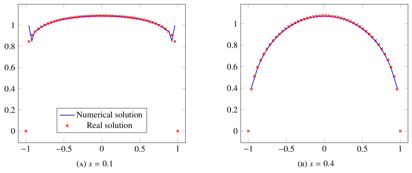
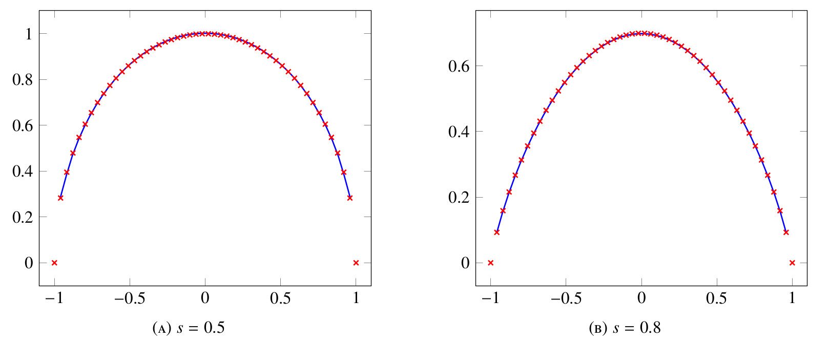
First of all, in order to test numerically the accuracy of our method for the discretization of the elliptic equation (1) we use the following problem
\begin{align}\label{PE_real}
\left\{\begin{array}{ll}
\fl{s}{u} = 1, & x\in(-L,L)
\\
u\equiv 0, & x\in\RR\setminus(-L,L).
\end{array}\right.
\end{align}
In this particular case, the solution can be expressed as follows
\begin{align}\label{real_sol}
u(x)=\frac{2^{-2s}\sqrt{\pi}}{\Gamma\left(\frac{1+2s}{2}\right)\Gamma(1+s)}\Big(L^2-x^2\Big)^s.
\end{align}
In figure 1 and figure 2, we show a comparison for different values of $s$ between the exact solution (8) and the computed numerical approximation. Here we consider $L=1$ and $N=50$. One can notice that, when $s=0.1$, the computed solution is to a certain extent different from the exact solution. However, one should be careful with such result and a more precise analysis of the error should be carried.
In figure 3, we present the computational errors evaluated for different values of $s$ and $h$.
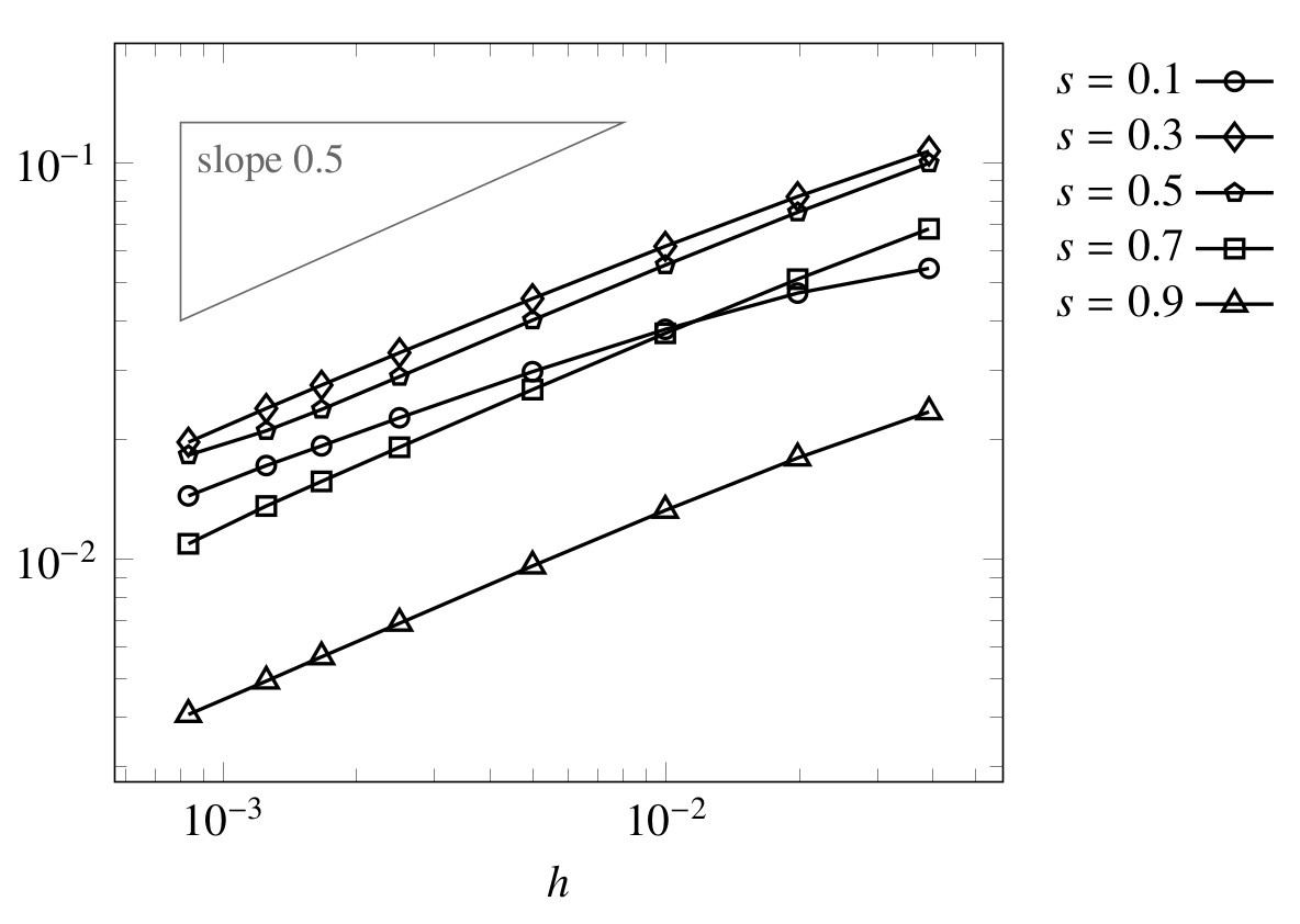
The rates of convergence shown are of order (in $h$) of $1/2$. This is in accordance with the known theoretical results (see, e.g., [1,Theorem 4.6]). One can see that the convergence rate is maintained also for small values of $s$. Since it is well-known that the notion of trace is not defined for the spaces $H^s(-L,L)$ with $s\leq 1/2$, it is somehow natural that we cannot expect a point-wise convergence in this case.
Control experiments
We present some numerical results for the controllability of the fractional heat equation (3). We use the finite-element approximation of $\fl{s}{}$ for the space discretization and the implicit Euler scheme in the time variable. We choose the penalization term ε as a function of h. A practical rule ([2]) is to choose $\phi(h)\sim h^{2p}$ where $p$ is the order of accuracy in space of the numerical method used for the discretization of the spatial operator involved. In this case, we take $p=1/2$.
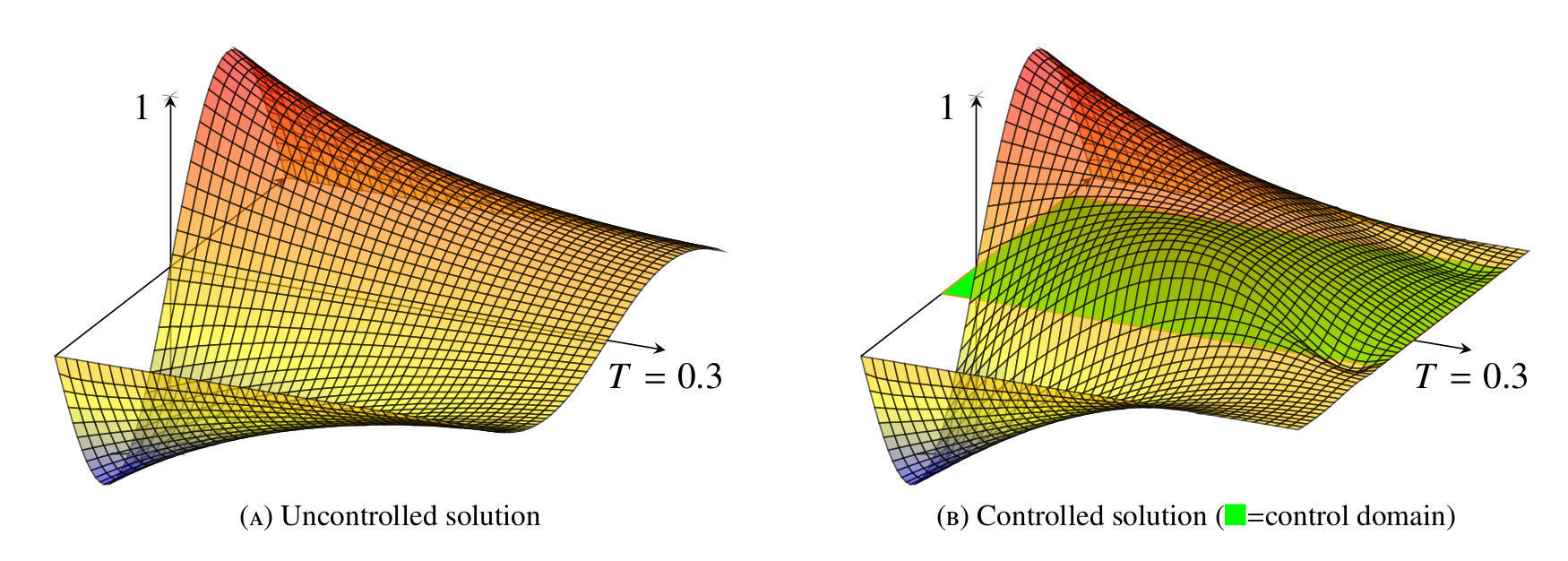
In figure 4, we observe the time evolution of the uncontrolled solution as well as the controlled solution. Here, we set $s=0.8$, $\omega=(-0.3,0.8)$ and $T=0.3$, and choose $z_0(x) = \sin(\pi x)$. The control domain is the highlighted zone on the plane $(t,x)$. As expected, we observe that the uncontrolled solution decays with time, but does not reach zero at time $T$, while the controlled solution does.
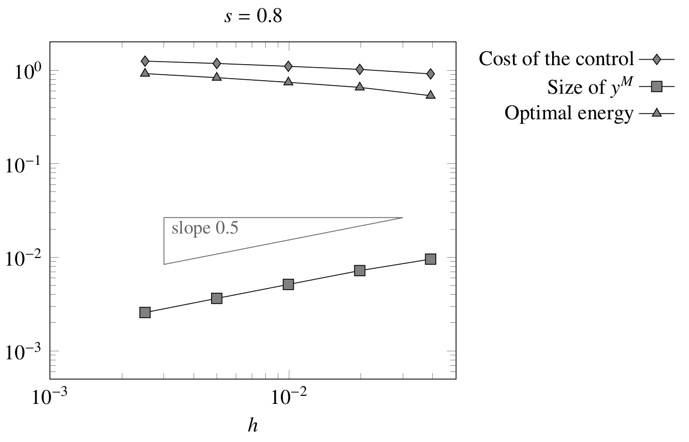
In figure 5, for $s=0.8$ we present the computed values of various quantities of interest when the mesh size goes to zero. More precisely, we observe that the control cost and the optimal energy remain bounded as $h\to 0$. On the other hand, we see that
\begin{align}\label{control_norm_behavior}
|y(T)|_{L^2(-1,1)}\,\sim\,C\sqrt{\phi(h)}=Ch^{1/2}.
\end{align}
We know that, for $s=0.8$, system (3) is null controllable. This is now confirmed by (9), according to [2,Theorem 1.7]. In fact, the same experiment can be repeated for different values of $s>1/2$, obtaining the same conclusions.
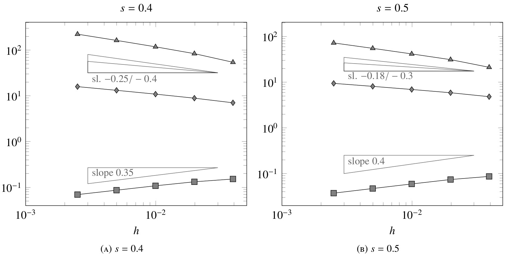
In figure 6, we illustrate the numerical results for the case $s\leq 1/2$. We observe that the cost of the control and the optimal energy increase in both cases, while the target $y(T)$ tends to zero with a slower rate than $h^{1/2}$. This seems to confirm that a uniform observability estimate for (3) does not hold and that we can only expect to have approximate controllability.
VIDEOS:
- Uncontrolled dynamics with s = 0.8 and T = 0.2 s – the solution dissipates but the zero state is not reached.
- Controlled dynamics with s = 0.8, T = 0.2 s and \omega = (−0.3, 0.8) – the zero state is reached.
MATLAB CODE:
- Matlab code for prog_control.m:
%%%%%%%%%%%%%%%%%%%%%%%%%%%%%%%%%%%%%%%%%%%%%%%%%%%%%%%%%%%%%%%%%%%%%%%%%%% %%%% Controllability of the fractional heat equation %%%%%%% %%%% %%%%%%% %%%% u_t + (-d_x^2)^s u = f, (x,t) in (-1,1)x(0,T) %%%%%%% %%%% u=0, (x,t) in [R\(-1,1)]x(0,T) %%%%%%% %%%% u(0)=u_0, x in (-1,1) %%%%%%% %%%% %%%%%%% %%%% using finite element and the penalized HUM %%%%%%% %%%% U. Biccari, V. Hernández-SantamarÃa, July 2017 %%%%%%% %%%% Heavily based on F. Boyer's work %%%%%%% %%%% v. 0.0 %%%%%%% %%%%%%%%%%%%%%%%%%%%%%%%%%%%%%%%%%%%%%%%%%%%%%%%%%%%%%%%%%%%%%%%%%%%%%%%%%% clear all clc separation='==================================================\n'; %prechoixN = [50]; %%%%%%%%%%%%%%%%%%%%%%%%%%%%%%%%%%%%%%%%%%%%%%%%%%%%%%%%%%%%%%%%%%%%%%%%%%% %%%% Load necessary functions %%%%%%%%%%%%%%%%%%%%%%%%%%%%%%%%%%%%%%%%%%%%%%%%%%%%%%%%%%%%%%%%%%%%%%%%%%% global donnees; m_donnees_control; maillages_control; maillage_uniforme=maill_funcs{1}; calcul_norme_Eh=maill_funcs{2}; produitscalaire_Eh=maill_funcs{3}; calcul_matrices_masse=maill_funcs{4}; evaluation_simple=maill_funcs{5}; schemas_control; init_matrices=schm_func{1}; solution_forward=schm_func{4}; solution_adjoint=schm_func{5}; HUM=schm_func{7}; grad_conj=schm_func{8}; lecture_donnees_control; for Nmaillage=choixN [maillage]=maillage_uniforme(Nmaillage); maillage=calcul_matrices_masse(maillage); y0=evaluation_simple(maillage.xi,donnees.y0); target=0*y0; for Mtemps=choixMtemps discr.Mtemps=Mtemps; matrices=init_matrices(maillage,discr); soly_libre=solution_forward(y0,zeros(size(y0,1),discr.Mtemps+1),... donnees,discr,matrices); sec_membre=-soly_libre(:,discr.Mtemps+1); for epsilon=choix_epsilon if (isfield(donnees,'phi') && (length(donnees.phi)>0)) h=maillage.pas; fprintf('epsilon=phi(h)= %s \n',donnees.phi); epsilon=eval(donnees.phi); end [phi0opt,it]=grad_conj(maillage,discr,donnees,matrices,... sec_membre,epsilon,donnees.tolerance,'oui',0*sec_membre); solphi=solution_adjoint(phi0opt,maillage,discr,donnees,matrices); controle=matrices.B*solphi; soly=solution_forward(y0,solphi,donnees,discr,matrices); cout_controle_temps=zeros(discr.Mtemps,1); for j=1:discr.Mtemps cout_controle_temps(j)=calcul_norme_Eh(maillage,controle(:,j),0); end fprintf(separation); fprintf("Size of the controlled solution at time T: %4.2e\n",... calcul_norme_Eh(maillage,soly(:,discr.Mtemps+1),0)); fprintf("Size of the uncontrolled solution at time T: %4.2e\n",... calcul_norme_Eh(maillage,soly_libre(:,discr.Mtemps+1),0)); F_eps=1/2*sum(cout_controle_temps.^2)*donnees.T/discr.Mtemps... +1/(2*epsilon)*calcul_norme_Eh(maillage,soly(:,discr.Mtemps+1),0).^2; fprintf('F_eps(v_eps)= %g \n',F_eps); J_eps=1/2*sum(cout_controle_temps.^2)*donnees.T/discr.Mtemps+... epsilon/2*calcul_norme_Eh(maillage,phi0opt,0)^2+... produitscalaire_Eh(maillage,solphi(:,1),y0,0); fprintf('-J_eps(q_eps)= %g \n',J_eps); fprintf('F_(v_opt)~J(mu_opt)= %g \n',abs(F_eps+J_eps)/(abs(F_eps)+abs(J_eps))); end end end % **para debug error('toto') % % *********************** % ***CHECKING THE SYMETRY % *********************** % psi=rand(size(y0,1),1); psitilde=rand(size(y0,1),1); Lambda_psi=HUM(psi,maillage,discr,donnees,matrices); Lambda_psitilde=HUM(psitilde,maillage,discr,donnees,matrices); disp(produitscalaire_Eh(maillage,psi,Lambda_psitilde,0)) disp(produitscalaire_Eh(maillage,psitilde,Lambda_psi,0)) disp(produitscalaire_Eh(maillage,psi,Lambda_psitilde,0)... -produitscalaire_Eh(maillage,psitilde,Lambda_psi,0))
- Matlab code for m_donnees_control.m:
default_tolerance = 10^(-8); % Default tolerance CG method

cas_test=cell(0);

cas_test{(end+1)} = struct('nom', 'Controllability fractional heat eq. s=0.5',...
		     'nbeq', 1,...
		     'nbc', 1,...
             'T', 0.5,...,
             'param_s', 0.5,...
		     'mat_B', @(x) intervalle(x,-0.3,0.8),...
             'y0', @(x) sin(pi.*x),...
             'maillage','uniforme',...
             'phi', 'h^4',... %penalization parameter
             'methode', 'euler');

cas_test{(end+1)} = struct('nom', 'Controllability fractional heat eq. s=0.8',...
		     'nbeq', 1,...
		     'nbc', 1,...
             'T', 0.5,...,
             'param_s', 0.8,...
		     'mat_B', @(x) intervalle(x,-0.3,0.8),...
             'y0', @(x) sin(pi.*x),...
             'maillage','uniforme',...
             'phi', 'h^4',... %penalization parameter
             'methode', 'euler');

fh=localfunctions;

function [y]=intervalle(x,a,b)
    y=(x>=a).*(x<=b);
end
- Matlab code for maillages_control.m:
%%%%%%%%%%%%%%%%%%%%%%%%%%%%%%%%%%%%%%%%%%%%%%%%%%%%%%%%%%%%%%%%%%%%%%%%%%%
%%%%%%%%%%%%%%%%%%%%%%%%%%%%%%%%%%%%%%%%%%%%%%%%%%%%%%%%%%%%%%%%%%%%%%%%%%%
%%%% Discretization of the domain                                        %%
%%%%       \Omega = (-1,1) in the elliptic case                          %%
%%%%       Q = (-1,1)x(0,T) in the parabolic case                        %%
%%%%       Space discretization: finite element                          %%
%%%%       Time discretization: implicit euler                           %%
%%%%%%%%%%%%%%%%%%%%%%%%%%%%%%%%%%%%%%%%%%%%%%%%%%%%%%%%%%%%%%%%%%%%%%%%%%%
%%%%%%%%%%%%%%%%%%%%%%%%%%%%%%%%%%%%%%%%%%%%%%%%%%%%%%%%%%%%%%%%%%%%%%%%%%%

%%%%%%%%%%%%%%%%%%%%%%%%%%%%%%%%%%%%%%%%%%%%%%%%%%%%%%%%%%%%%%%%%%%%%%%%%%%
%%%% Uniform mesh 1D
%%%%%%%%%%%%%%%%%%%%%%%%%%%%%%%%%%%%%%%%%%%%%%%%%%%%%%%%%%%%%%%%%%%%%%%%%%%

maill_funcs=localfunctions;

function [maillage] = maillage_uniforme(N)

    x=linspace(-1,1,N+2)';

    himd = x(2:end-1)-x(1:end-2);
    hipd = x(3:end)-x(2:end-1);
    hi = 0.5*(hipd+himd);
    x = x(2:end-1);

    maillage=struct('nom','maillage uniforme',...
    'dim',1,...
    'xi',x,...
    'hi',hi,...
    'pas',max(hi),...
    'N',N);

end

%%%%%%%%%%%%%%%%%%%%%%%%%%%%%%%%%%%%%%%%%%%%%%%%%%%%%%%%%%%%%%%%%%%%%%%%%%%
%%%%
%%%% Norm in the discrete state space Eh
%%%%
%%%%%%%%%%%%%%%%%%%%%%%%%%%%%%%%%%%%%%%%%%%%%%%%%%%%%%%%%%%%%%%%%%%%%%%%%%%

function [n]=calcul_norme_Eh(m,vecteur,s)

    n = sqrt(produitscalaire_Eh(m,vecteur,vecteur,s));

end

%%%%%%%%%%%%%%%%%%%%%%%%%%%%%%%%%%%%%%%%%%%%%%%%%%%%%%%%%%%%%%%%%%%%%%%%%%%
%%%%
%%%% Scalr product in the discrete state space Eh
%%%%
%%%%%%%%%%%%%%%%%%%%%%%%%%%%%%%%%%%%%%%%%%%%%%%%%%%%%%%%%%%%%%%%%%%%%%%%%%%

function [n]=produitscalaire_Eh(maill,vecteur,vecteur2,s)

    switch s
        case 0
            n=vecteur'*maill.H_Eh*vecteur2;
    end

    end

%%%%%%%%%%%%%%%%%%%%%%%%%%%%%%%%%%%%%%%%%%%%%%%%%%%%%%%%%%%%%%%%%%%%%%%%%%%
%%%%
%%%%  Storage of the mesh size parameters (needed for non-uniform meshes)
%%%%
%%%%%%%%%%%%%%%%%%%%%%%%%%%%%%%%%%%%%%%%%%%%%%%%%%%%%%%%%%%%%%%%%%%%%%%%%%%

function [maill]=calcul_matrices_masse(m)

    global donnees;
    maill=m;

        bloc=sparse(maill.N,maill.N);
        maill.H_Eh=sparse(maill.N*donnees.nbeq,maill.N*donnees.nbeq);
        maill.H_Uh=sparse(maill.N*donnees.nbc,maill.N*donnees.nbc);

        for i=1:maill.N
            bloc(i,i)=maill.hi(i);
        end

        for j=1:donnees.nbeq
            maill.H_Eh( 1+(j-1)*maill.N:j*maill.N , 1+(j-1)*maill.N:j*maill.N )=bloc;
        end

        for j=1:donnees.nbc
            maill.H_Uh( 1+(j-1)*maill.N:j*maill.N , 1+(j-1)*maill.N:j*maill.N )=bloc;
        end

end

%%%%%%%%%%%%%%%%%%%%%%%%%%%%%%%%%%%%%%%%%%%%%%%%%%%%%%%%%%%%%%%%%%%%%%%%%%%
%%%%
%%%%  Evaluation of a given function on a mesh
%%%%
%%%%%%%%%%%%%%%%%%%%%%%%%%%%%%%%%%%%%%%%%%%%%%%%%%%%%%%%%%%%%%%%%%%%%%%%%%%

function [v]=evaluation_simple(points,f)
    v=zeros(size(points,1),1);

    if isnumeric(f)
        v=f*(1+v);
    elseif isa(f,'function_handle')
        v=feval(f,points);
    else
        disp('Erreur dans le type d''argument passe a evaluation_simple')
    end
end
- Matlab code for schemas_control.m:
%%%%%%%%%%%%%%%%%%%%%%%%%%%%%%%%%%%%%%%%%%%%%%%%%%%%%%%%%%%%%%%%%%%%%%%%%%%
%%%%  Initialization of the matrices needed in the code
%%%%  A = rigidity matrix
%%%%  B = control operator
%%%%  C = matrix of the implicit Euler method
%%%%  M = mass matrix
%%%%%%%%%%%%%%%%%%%%%%%%%%%%%%%%%%%%%%%%%%%%%%%%%%%%%%%%%%%%%%%%%%%%%%%%%%%

schm_func=localfunctions;

function [matrices,maillage]=init_matrices(maillage,discr)

    global donnees

    matrices=struct();
    matrices.B=construction_matrice_B(maillage,donnees);
    matrices.A=construction_matrice_A(maillage,donnees);

    dt=donnees.T/discr.Mtemps;

    M=2/3*eye(maillage.N);
    for i=2:maillage.N-1
        M(i,i+1)=1/6;
        M(i,i-1)=1/6;
    end
    M(1,2)=1/6;
    M(maillage.N,maillage.N-1)=1/6;

    M=maillage.pas*sparse(M);
    matrices.M=M;

    matrices.C=speye(maillage.N,maillage.N)+dt*(matrices.M\matrices.A);
end


%%%%%%%%%%%%%%%%%%%%%%%%%%%%%%%%%%%%%%%%%%%%%%%%%%%%%%%%%%%%%%%%%%%%%%%%%%%
%%%%  Construction of the matrix A (fractional Laplacian)
%%%%%%%%%%%%%%%%%%%%%%%%%%%%%%%%%%%%%%%%%%%%%%%%%%%%%%%%%%%%%%%%%%%%%%%%%%%

function [A]=construction_matrice_A(maillage,donnees)

         A=fl_rigidity(donnees.param_s,1,maillage.N);
end

%%%%%%%%%%%%%%%%%%%%%%%%%%%%%%%%%%%%%%%%%%%%%%%%%%%%%%%%%%%%%%%%%%%%%%%%%%%
%%%% Construction of the matrix B
%%%%%%%%%%%%%%%%%%%%%%%%%%%%%%%%%%%%%%%%%%%%%%%%%%%%%%%%%%%%%%%%%%%%%%%%%%%

% function [B]=construction_matrice_B(maillage,donnees)
%
%         B=sparse(maillage.N*donnees.nbeq,maillage.N*donnees.nbc);
%
%         bloc=sparse(maillage.N,maillage.N);
%
%             for j=1:donnees.nbeq
%                 for k=1:donnees.nbc
%                     controlejk=evaluation_simple(maillage.xi,donnees.mat_B);
%
%                     bloc=diag(controlejk);
%
%                     B( 1+(j-1)*maillage.N:j*maillage.N ,...
%                         1+(k-1)*maillage.N:k*maillage.N )=bloc;
%                 end
%             end
%
% end

function [B]=construction_matrice_B(maillage,donnees)

        aux = sparse(maillage.N*donnees.nbeq,maillage.N*donnees.nbc);

        bloc=sparse(maillage.N,maillage.N);

            for j=1:donnees.nbeq
                for k=1:donnees.nbc
                    controlejk=evaluation_simple(maillage.xi,donnees.mat_B);

                    bloc=diag(controlejk);

                    aux( 1+(j-1)*maillage.N:j*maillage.N ,...
                        1+(k-1)*maillage.N:k*maillage.N )=bloc;
                end
            end

        B=sparse(maillage.N*donnees.nbeq,maillage.N*donnees.nbc);


        for i=2:maillage.N-1
            B(i,i) = maillage.pas;
            B(i,i+1) = 0.5*maillage.pas;
            B(i,i-1) = 0.5*maillage.pas;
        end
        B(1,1) = maillage.pas;
        B(1,2) = 0.5*maillage.pas;
        B(maillage.N,maillage.N-1) = 0.5*maillage.pas;
        B(maillage.N,maillage.N) = maillage.pas;

        B = aux*B;
end


%%%%%%%%%%%%%%%%%%%%%%%%%%%%%%%%%%%%%%%%%%%%%%%%%%%%%%%%%%%%%%%%%%%%%%%%%%%
%%%% Solution to the direct problem
%%%%
%%%% u_t + (-d_x^2)^s u = f, (x,t) in (-1,1)x(0,T)
%%%% u=0,                    (x,t) in [R\(-1,1)]x(0,T)
%%%% u(0)=u_0,                x in (-1,1)
%%%%
%%%% using implicit Euler method
%%%%%%%%%%%%%%%%%%%%%%%%%%%%%%%%%%%%%%%%%%%%%%%%%%%%%%%%%%%%%%%%%%%%%%%%%%%

function [soly]=solution_forward(y0,adjoint,donnees,discr,matrices)

        soly=zeros(size(y0,1),discr.Mtemps+1);
        dt=donnees.T/discr.Mtemps;
        soly(:,1)=y0;
        for i=1:discr.Mtemps
            soly(:,i+1)=matrices.C\(soly(:,i) ...
				  + dt*matrices.B*matrices.B'*adjoint(:,i));
        end
end

%%%%%%%%%%%%%%%%%%%%%%%%%%%%%%%%%%%%%%%%%%%%%%%%%%%%%%%%%%%%%%%%%%%%%%%%%%%
%%%% Solution to the adjoint problem
%%%%
%%%% -v_t + (-d_x^2)^s v = 0, (x,t) in (-1,1)x(0,T)
%%%% v=0,                     (x,t) in [R\(-1,1)]x(0,T)
%%%% v(T)=v_T,                 x in (-1,1)
%%%%
%%%% using implicit Euler method
%%%%%%%%%%%%%%%%%%%%%%%%%%%%%%%%%%%%%%%%%%%%%%%%%%%%%%%%%%%%%%%%%%%%%%%%%%%

function [solphi]=solution_adjoint(phi0,maillage,discr,donnees,matrices)

        solphi=zeros(size(phi0,1),discr.Mtemps+1);
        solphi(:,discr.Mtemps+1) = phi0;
        for i=discr.Mtemps:-1:1
            solphi(:,i)=matrices.C\solphi(:,i+1);
        end
end

%%%%%%%%%%%%%%%%%%%%%%%%%%%%%%%%%%%%%%%%%%%%%%%%%%%%%%%%%%%%%%%%%%%%%%%%%%%
%%%%
%%%%  Finite Element approximation of the fractional Laplacian on (-L,L)
%%%%
%%%%%%%%%%%%%%%%%%%%%%%%%%%%%%%%%%%%%%%%%%%%%%%%%%%%%%%%%%%%%%%%%%%%%%%%%%%

function A = fl_rigidity(s,L,N)

x = linspace(-L,L,N+2);
x = x(2:end-1);
h = x(2)-x(1);

A = zeros(N,N);
%
% for i=2:N-1
%     A(i,i) = 2;
%     A(i,i+1) = -1;
%     A(i,i-1) = -1;
% end
%
% A(1,1) = 2;
% A(1,2) = -1;
% A(N,N-1) = -1;
% A(N,N) = 2;
%
% A = (1/h)*sparse(A);

%  Normalization constant of the fractional Laplacian

c = (s*2^(2*s-1)*gamma(0.5*(1+2*s)))/(sqrt(pi)*gamma(1-s));

%  Elements A(i,j) with |j-i|>1

for i=1:N-2
    for j=i+2:N
        k = j-i;
        if s==0.5 && k==2
            A(i,j) = 56*log(2)-36*log(3);
        elseif s==0.5 && k~=2
            A(i,j) = -(4*((k+1)^2)*log(k+1)+4*((k-1)^2)*log(k-1)...
                -6*(k^2)*log(k)-((k+2)^2)*log(k+2)-((k-2)^2)*log(k-2));
        else
            P = 1/(4*s*(1-2*s)*(1-s)*(3-2*s));
            q = 3-2*s;
            B = P*(4*(k+1)^q+4*(k-1)^q-6*k^q-(k-2)^q-(k+2)^q);
            A(i,j) = -2*h^(1-2*s)*B;
        end
    end
end

%  Elements of A(i,j) with j=1+1 ----- upper diagonal

for i=1:N-1
    if s==0.5
       A(i,i+1) = 9*log(3)-16*log(2);
    else
       A(i,i+1) = h^(1-2*s)*((3^(3-2*s)-2^(5-2*s)+7)/(2*s*(1-2*s)*(1-s)*(3-2*s)));
    end
end

A = A+A';

%  Elements on the diagonal

for i=1:N
    if s==0.5
       A(i,i) = 8*log(2);
    else
       A(i,i) = h^(1-2*s)*((2^(3-2*s)-4)/(s*(1-2*s)*(1-s)*(3-2*s)));
    end
end

A = c*A;

end

%%%%%%%%%%%%%%%%%%%%%%%%%%%%%%%%%%%%%%%%%%%%%%%%%%%%%%%%%%%%%%%%%%%%%%%%%%%
%%%%
%%%%  Implementation of the penalized HUM (see F. Boyer - On the penalized
%%%%  HUM approach and its application to the numerical approximation of
%%%%  null-controls for parabolic problems)
%%%%
%%%%%%%%%%%%%%%%%%%%%%%%%%%%%%%%%%%%%%%%%%%%%%%%%%%%%%%%%%%%%%%%%%%%%%%%%%%

function [w] = grammian(phi0,maillage,discr,donnees,matrices)

    solphi=solution_adjoint(phi0,maillage,discr,donnees,matrices);
    soly= solution_forward(0*phi0,solphi,donnees,discr,matrices);

    w=soly(:,discr.Mtemps+1);

end

function [f,it]=grad_conj(maillage,discr,donnees,matrices,secmem,epsilon,tol,verbose,f_init)

    maillages_control;
        calcul_norme_Eh=maill_funcs{2};
        produitscalaire_Eh=maill_funcs{3};

    it_restart=5000;
    f=f_init;

    Lambdaf=grammian(f,maillage,discr,donnees,matrices);

    g = Lambdaf - secmem;

    g=g+epsilon*f;

    w=g;

    erreurinit=calcul_norme_Eh(maillage,g,0);
    normeinit=calcul_norme_Eh(maillage,secmem,0);


    erreurtemps=[erreurinit];

    erreur_gradconj=10*tol;
    it=0;

    tic
    while (erreur_gradconj>tol)

        it=it+1;

        Lambdaw=grammian(w,maillage,discr,donnees,matrices);

	    newg = Lambdaw + epsilon*w;

        rho = produitscalaire_Eh(maillage,g,g,0)/ ...
        produitscalaire_Eh(maillage,newg,w,0);
        f=f-rho*w;
        newg = g - rho*newg;

        erreur_gradconj=calcul_norme_Eh(maillage,newg,0)/erreurinit;

        if (erreur_gradconj>tol)

            gam=produitscalaire_Eh(maillage,newg,newg,0)/ ...
                produitscalaire_Eh(maillage,g,g,0);

            if (mod(it,it_restart)==0)
                gam=0;
            end
            w=newg+ gam*w;
        end
        g=newg;
        fprintf("Iteration %g - Error %4.3e \n",it,erreur_gradconj);

        if verbose=='oui'
            if (mod(it,500)==0)
                fprintf('Iteration %g - Error %4.3e - Time: %d seconds\n',it,erreur_gradconj,round(toc()));
            end
        end

    end

    Lambdaf=grammian(f,maillage,discr,donnees,matrices);
    w = Lambdaf - secmem;
    w = w + epsilon * f;

    fprintf('Gap = %s \n',string(calcul_norme_Eh(maillage,w,0)));

end

%%%%%%%%%%%%%%%%%%%%%%%%%%%%%%%%%%%%%%%%%%%%%%%%%%%%%%%%%%%%%%%%%%%%%%%%%%%
%%%%
%%%%  Evaluation of a given function on a mesh
%%%%
%%%%%%%%%%%%%%%%%%%%%%%%%%%%%%%%%%%%%%%%%%%%%%%%%%%%%%%%%%%%%%%%%%%%%%%%%%%

function [v]=evaluation_simple(points,f)
    v=zeros(size(points,1),1);

    if isnumeric(f)
        v=f*(1+v);
    elseif isa(f,'function_handle')
        v=feval(f,points);
    else
        disp('Erreur dans le type d''argument passe a evaluation_simple')
    end
end
- Matlab code for lecture_donnees_control.m:
%%%%%%%%%%%%%%%%%%%%%%%%%%%%%%%%%%%%%%%%%%%%%%%%%%%%%%%%%%%%%%%%%%%%%%%%%%%
%%%%
%%%% Paramaters for the time discretization
%%%%
%%%%%%%%%%%%%%%%%%%%%%%%%%%%%%%%%%%%%%%%%%%%%%%%%%%%%%%%%%%%%%%%%%%%%%%%%%%

discr=cell(0);

discr{(end+1)} = struct('methode','elliptic',...
                        'Mtemps',0,...
                        'theta',0....
                       );

discr{(end+1)} = struct('methode','euler',...
                        'Mtemps',100,...
                        'theta',0....
                       );

%%%%%%%%%%%%%%%%%%%%%%%%%%%%%%%%%%%%%%%%%%%%%%%%%%%%%%%%%%%%%%%%%%%%%%%%%%%
%%%%
%%%% Reading of the datas
%%%%
%%%%%%%%%%%%%%%%%%%%%%%%%%%%%%%%%%%%%%%%%%%%%%%%%%%%%%%%%%%%%%%%%%%%%%%%%%%

fprintf(separation);
fprintf('Choice of the test case:\n');

fprintf(separation);
if exist('prechoix','var')
    choix=prechoix;
    printf("Choice number %g\n",choix);
else
        for i=1:length(cas_test)
                    temp=cell2mat(cas_test(1,i));
                    fprintf('%d) %s\n',i,temp.nom);
                    clear temp i
        end

        choix=input('Choose among the cases proposed: ');
        while double(choix)>length(cas_test)
            choix=input('Choose among the cases proposed: ');
        end
end
choix=double(choix);

donnees=cell2mat(cas_test(choix));

if ~isfield(donnees,'tolerance')
    donnees.tolerance=default_tolerance;
end

fprintf(separation);

choix_maillage=-1;
if isfield(donnees,'maillage')
    switch donnees.maillage
    case 'uniforme'
        choix_maillage=1;
        fprintf("Uniform mesh \n");
    end
end

switch choix_maillage
case 1
    donnees.maillage="uniforme";
end

fprintf(separation);

if(exist('prechoixN'))
    choixN=prechoixN;
else
    choixN=input('Number of dicretization points in space :');
    choixN=floor(double(choixN));
end

fprintf(separation);
choix=-1;
if isfield(donnees,'methode')

    for i=1:length(discr)
        if strcmp(discr{i}.methode,donnees.methode)
            choix=i;
            fprintf('Scheme in time: %s \n',donnees.methode);
        end
    end
end

if (choix==-1)

    fprintf('Choice of the scheme in time:\n');
    for i=1:length(discr)
        fprintf('%d) %s\n',i,discr{i}.methode);
    end

    choix=-1;
    while ((choix)<=0) || ((choix)>length(discr))
        choix=input('Choose:');
    end
    choix=floor(double(choix));

end

discr=discr{choix};

if strcmp(discr.methode,'elliptic')
    choixMtemps=0;

else
   fprintf(separation);
    if(exist("prechoixT"))
        choixMtemps=floor(double(prechoixT));
    else
        choixMtemps=input('Number of discretization points in time:');
        choixMtemps=floor(double(choixMtemps));
    end
end

if ~isfield(donnees,'pt_fixe_it_max')
    donnees.pt_fixe_it_max=50;
end

%%%%%%%%%%%%%%%%%%%%%%%%%%%%%%%%%%%%%%%%%%%%%%%%%%%%%%%%%%%%%%%%%%%%%%%%%%%
%%%%
%%%% Chioce of the penalization parameter
%%%%
%%%%%%%%%%%%%%%%%%%%%%%%%%%%%%%%%%%%%%%%%%%%%%%%%%%%%%%%%%%%%%%%%%%%%%%%%%%

fprintf(separation);

if ((isfield(donnees,'phi')) && (length(donnees.phi)>0))
    choix_epsilon=['1'];
elseif (isfield(donnees,'epsilon'))
    choix_epsilon=donnees.epsilon;
else
    choix_epsilon=input('Choice of epsilon :');
end
Bibliography
[1] Acosta, G., Bersetche, F. M., and Borthagaray, J. P. A short FE implementation for a 2d homogeneous Dirichlet problem of a Fractional Laplacian Comput. Math. Appl. (2017).
[2] Boyer, F On the penalized hum approach and its applications to the numerical approximation of null-controls for parabolic problems ESAIM: Proceedings vol. 41 (2013), pp. 15–58.
[3] Micu, S., and Zuazua, E. On the controllability of a fractional order parabolic equation. SIAM J. Control Optim., vol. 44, no. 6 (2006), pp. 1950–1972.
[4] Miller, L. On the controllability of anomalous diffusions generated by the fractional Laplacian. Math. Control Signals Systems, vol. 18, no. 3 (2006), pp. 260–271.

