
Spain 05.08.2022
Null Controllability of a Nonlinear Age, Space and Two-sex Structured Population Dynamics Model
Author: Yacouba Simpore
Motivation and description of two sex structured population dynamics model
Motivation
Malaria is a disease caused by parasites of the genus Plasmodium. According to the WHO, this disease causes approximately one million victims per year worldwide.

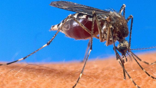
Figure 1. Anophel Gambiae
The parasite is transmitted to humans through the bite of an infected mosquito. These mosquitoes, “vectors” of malaria, all belong to the genus Anopheles.
In the fight against malaria and other diseases transmitted to humans by insects (such as the Anopheles Gambiae), many methods are used around the world (development of vaccines, etc.). In recent years, the mosquito control strategy is increasingly used in many countries such as the United States and West Africa.
[1] We have in west Africa “Target Malaria” project underway and which aims to drive the density of wild female mosquitoes to zero in long time horizon. The strategy involves three stages:• The first phase: Creation of sterile male mosquitoes. The researchers generated male Anopheles gambiae mosquitoes, which can reproduce with wild females, but which will not produce any offspring. This first release represents a test phase which will make it possible to acquire knowledge and build an operational capacity.
• The second phase: (Creation of self-limiting male mosquitoes) consists of releasing male mosquitoes leading to a distortion of the sex ratio of the targeted mosquito population. The purpose of this phase is to learn more about the development of their technology, using a line of self-limiting male mosquitoes, which will decline in number with each generation.
• The third stage or Gene Drive consists of the production of genetically modified, fertile mosquitoes, which can transmit a genetic modification to their offspring. This will be passed on to the following generations. They are currently investigating several options, the two most promising are :
– A genetically modified strain with fertile males that produce predominantly male offspring, leading to a distortion in the sex ratio of the targeted mosquito population;
– A genetically modified strain with fertile males carrying a gene that will spread through the mosquito population and cause females that inherit the gene from both parents to be sterile.
[2] In the coming months more than 2 million genetically modified mosquitoes will be released in Florida. The mosquitoes, created by biotech firm Oxitec, will be non-biting Aedes aegypti males engineered to only produce viable male offspring, per the company. Oxitec says the plan will reduce numbers of the invasive Aedes aegypti, which can carry diseases like Zika, yellow fever and dengue.
• In this blog we give mathematically some ideas on the possibility of controlling of mosquitoes population dynamics. For reasons like as the difference in lifespan between male mosquitoes (14 days) and female (30 days) and the difference in mortality functions, we preferred to work with the two-sex model which seems the best fit.
• In the strategies cited, the control methods used seem to be birth control or the combination of birth control and distributed control, in this first work, we will focus on distributed controls.
Description of two sex structured population dynamics model
We denote by \Xi=\omega\times(a_1,a_2)\times (0,T)\subset Q and \Xi'=\omega'\times(b_1,b_2)\times (0,T)\subset Q where Q=\Omega\times(0,A)\times(0,T). We denote also \Sigma=\partial\Omega\times(0,A)\times(0,T)\hbox{, }Q_T=\Omega\times(0,T) and Q_A=\Omega\times(0,A).
Let (m,f) solution of the following system :
\left\lbrace \begin{array}{ll} \dfrac{\partial m}{\partial t}+\dfrac{\partial m}{\partial a}-K_m\Delta m+\mu_m m=\chi_{\Xi}v_m&\text{ in }Q,\\ \dfrac{\partial f}{\partial t}+\dfrac{\partial f}{\partial a}-K_f\Delta f+\mu_f f=\chi_{\Xi'}v_f&\text{ in }Q,\\ m(\sigma,a,t)=f(\sigma,a,t)=0&\text{ on }\Sigma, \\ m(x,a,0)=m_0\quad f(x,a,0)=f_0&\text{ in }Q_A,\\ m(x,0,t)=(1-\gamma)N(x,t)\text{, }f(x,0,t)=\gamma N(x,t)& \text{ in }Q_T,\\ N(x,t)=\int_{0}^{A}\beta(a,M)fda\text{; } M=\int_{0}^{A}\lambda(a)mda & \text{ in }Q_T. \end{array} \right. (1.1)
where m_0\in L^2(Q_A), f_0\in L^2(Q_A), v_m\in L^2(Q), v_f\in L^2(Q) and \gamma\in(0,1).
The functions, m(x,a,t) and f(x,a,t) represent the density of males and females of age a at time t in position x, respectively.
We assume that the fertility functions \beta, \lambda and mortality \mu_m and \mu_f satisfy the following demographic properties:
(H_1): \left\lbrace \begin{array}{ll} (i)\hbox{ }\mu_m\geq 0, \quad \mu_f\geq 0\text{ a.e. in } [0,A], \\\ (ii)\hbox{ }\mu_m\in L_{loc}^{1}\left([0,A)\right),\quad \mu_f\in L_{loc}^{1}\left([0,A)\right), \\ (iii)\hbox{ }\int_{0}^{A}\mu_m(a)da=+\infty,\quad \int_{0}^{A}\mu_f(a)da=+\infty. \end{array} \right.
The functions
\Pi_{m}(a)=e^{-\int\limits_{0}^{a}\mu_m(s)ds}\text{ and }\Pi_{f}(a)=e^{-\int\limits_{0}^{a}\mu_f(s)ds}
denote the probability of survival of male individuals of age a and female individuals of age a, respectively.
(H_{2}): \left\lbrace \begin{array}{ll} (i)\hbox{ }\beta\in C\left([0,A]\times \mathbb{R}\right),\\ (ii)\hbox{ }\beta(a,p)\geq 0\text{ for all } (a,p)\in[0,A]\times \mathbb{R},\\ (iii)\hbox{ }\beta(a,0)=0\text{ in } (0,A). \end{array} \right.
(H_{3}): \left\lbrace \begin{array}{ll} \lambda\in C^{1}\left([0,A]\right),\\ \lambda\geq 0\text{ for all } a\in [0,A]. \end{array} \right.
Moreover, we suppose that:
(H_{4}):\left\lbrace \begin{array}{ll} (i)\hbox{ }\text{there exists }b\in (0,A)\text{ such that }\beta(a,p)=0, \forall (a,p)\in [0,b)\times\mathbb{R},\\ (ii)\hbox{ }\text{ there exists } L>0 \text{ such that }|\beta(a,p)-\beta(a,q)|\leq L|p-q|\\ \text{ for all } p, q \in\mathbb{R}\text{, } a\in [0,A],\\ (iii)\hbox{ }\text{there exists }\beta_{0}>0 \text{ such that } 0\leq\beta(a,p)\leq \beta_{0}\text{, } \forall (a,p)\in [0,A]\times\mathbb{R}. \end{array} \right. (1.2)
(H_5):\left\lbrace \begin{array}{ll} \lambda\mu_m\in L^{1}((0,A)).\\ \end{array} \right.
2 Null controllability
2.1 Null controllablity
We have the following
Theorem 2.1.
Suppose that the assumptions (H_1)-(H_2)-(H_3)-(H_4)-(H_5) hold. If (0,b)\cap(a_1,a_2)\cap(b_1,b_2)\neq \emptyset, for every time T>\max\{a_1,b_1\}+\max\{A-a_2,A-b_2\} and for every (m_0,f_0)\in \left(L^2(Q_A)\right)^2, there exists (v_m,v_f)\in L^2(\Xi)\times L^2(\Xi') such the solution (m,f) of the system (1.1) verifies:
m(x,a,T)=0 \hbox{ a.e. } x\in \Omega, \hbox{ } a\in (0,A), (2.1)
f(x,a,T)=0 \hbox{ a.e. } x\in \Omega,\hbox{ } a\in (0,A). (2.2)
Remark 2.1.
Notice that \omega\cap \omega' can be empty
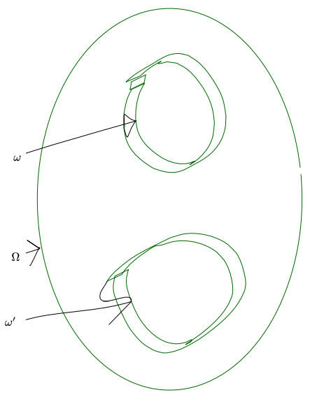
Figure 2.Illustration of the control support in space
The following figure gives an estimate of the time in the case of an extreme method of controllability
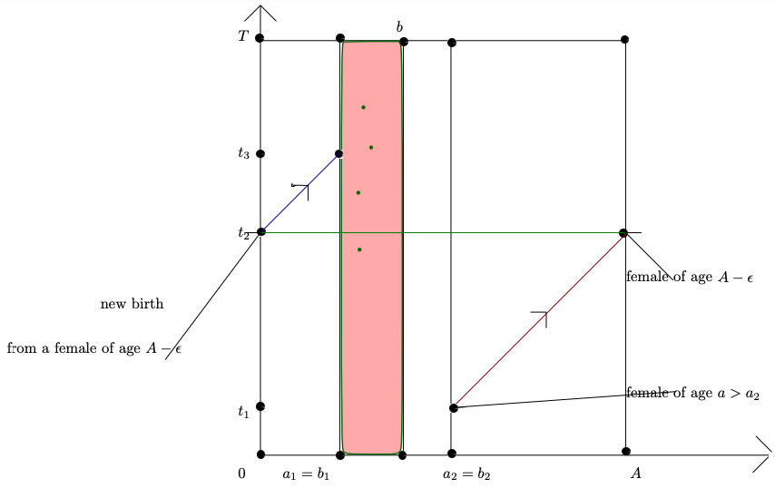
Figure 3.The method being to eliminate all male and female individuals whose age is between a_1 and a_2 (t_3-t_1=A-a_2+\epsilon+a_1).In this case, all males and females whose age is greater than a_2 can live to the maximum age A and can have offspring which can also live to the age of a_1.
2.2 Null controllability of auxiliary system
Let p be a function in L^{2}(Q_T), we define the auxilliary system given by:
\left\lbrace \begin{array}{ll} \dfrac{\partial m}{\partial t}+\dfrac{\partial m}{\partial a}-K_m\Delta m+\mu_m m=\chi_{\Xi}v&\text{ in }Q ,\\ \dfrac{\partial f}{\partial t}+\dfrac{\partial f}{\partial a}-K_f\Delta f+\mu_f f=\chi_{\Xi'}u&\text{ in }Q,\\ m(\sigma,a,t)=f(\sigma,a,t)=0&\text{ on }\Sigma, \\ m(x,a,0)=m_0\quad f(x,a,0)=f_0 &\text{ in }Q_A,\\ m(x,0,t)=(1-\gamma)\int_{0}^{A}\beta(a,p)fda,\\ f(x,0,t)=\gamma \int_{0}^{A}\beta(a,p)fda& \text{ in }Q_T.\\ \end{array} \right. (2.3)
The system (2.3) admits a unique solution (m,f)\in (L^2((0,A)\times (0,T);H^{1}_{0}(\Omega)))^2 and the system (2.3) is null controllable for every T>\max\{a_1,b_1\}+\max\{A-a_2,A-b_2\}. Moreover the null controllability of the system (2.3) is equivalent of the Observability inequality. Let (n,l) be the solution of the following adjoint system to the auxilliary system (2.3)
\left\lbrace \begin{array}{ll} -\dfrac{\partial n}{\partial t}-\dfrac{\partial n}{\partial a}-K_m\Delta n+\mu_m n=0 &\text{ in }Q ,\\ -\dfrac{\partial l}{\partial t}-\dfrac{\partial l}{\partial a}-K_f\Delta l+\mu_f l=(1-\gamma)\beta(a,p)n(x,0,t)+\gamma\beta(a,p)l(x,0,t)&\text{ in }Q,\\ n(\sigma,a,t)=l(\sigma,a,t)=0&\text{ on }\Sigma, \\ n(x,a,T)=n_T\quad l(x,a,T)=l_T&\text{ in }Q_A,\\ n(x,A,t)=0,\quad l(x,A,t)=0& \text{ in }Q_T.\\ \end{array} \right. (2.4)
Under the assumptions on the time T, we have the following:
2.3 Observability Inequality
Theorem 2.2
Under the assumptions of Theorem 1, for every T>\max\{a_1,b_1\}+\max\{A-a_2,A-b_2\}, there exists a constant C_{T}>0 independent of p such that the solution (n,l) of the system (2.4) verifies:
\int_{0}^{A}\int_{\Omega}n^2(x,a,0)dxda+\int_{0}^{A}\int_{\Omega}l^2(x,a,0)dxda
\leq C_{T}\left(\int_{\Xi}n^2(x,a,t)dxdadt+\int_{\Xi'}l^2(x,a,t)dxdadt\right).
2.4 Representation for the solution of the adjoint system
The idea to establish the observability inequality is the estimation of the non local terms of the adjoint system. For this reason, we first begun to formulating a representation of the solution of cascade adjoint system by caractheristics method and semigroup.
For (n_T,l_T)\in(L^2(Q_A))^2, under the assumptions (H_1) and (H_2), the cascade system (2.4) admits a unique solution (n,l). Moreover, integrating along the characteristics line the solution (n,l) of (2.4) is given by:
n(t) = \begin{cases} \dfrac{\pi_1(a+T-t)}{\pi_1(a)}e^{(T-t) K_m\Delta} n_T(x,a+T-t) \text{ if } T-t \leq A-a, \\ 0 \text{ if } A-a \lt T-t, \end{cases} (2.5)
and
l(t)= \begin{cases} \scriptstyle \frac{\pi_2(a+T-t)}{\pi_2(a)}e^{(T-t) K_f\Delta}l_T(x,a+t-T)\\ \scriptstyle +\int_{t}^{T}\frac{\pi_2(a+s-t)}{\pi_2(a)}e^{(s-t) K_f\Delta}\beta(a+s-t,p(x,s))\left((1-\gamma)n(x,0,s)+\gamma l(x,0,s)\right)ds\text{ in } D_1, \\ \scriptstyle \int_{t}^{t+A-a}\frac{\pi_2(a+s-t)}{\pi_2(a)}e^{(s-t) K_f\Delta}\beta(a+s-t,p(x,s))\left((1-\gamma)n(x,0,s)+\gamma l(x,0,s)\right)ds \text{ in } D_2, \end{cases} (2.6)
where \pi_1(a)=e^{-\int_{0}^{a}\mu_m(r)dr}\text {, }\pi_2(a)=e^{-\int_{0}^{a}\mu_f(r)dr}\text{, } e^{tK_m \Delta} is the semigroup of -K_m\Delta with the Dirichlet boundary condition and
D_1=\{(a,t)\in (0,A)\times (0,T) \text{ such that } T-t\leq A-a\},
D_2=\{(a,t)\in (0,A)\times (0,T) \text{ such that } T-t > A-a\}.
Using the fact that \beta(a,p)=0\hbox{ for all }a\in[0,b). We establish the following:
2.4.1 Estimations of the non-local terms
Proposition 2.1.
Under the assumptions of Theorem 1, for every \eta satisfying a_1 \lt \eta \lt T, there exists C>0 such that the following inequality
\int_{0}^{T-\eta}\int_{\Omega}n^2(x,0,t)dxdt\leq C\int_{0}^{T}\int_{a_1}^{a_2}\int_{\omega}n^2(x,a,t)dxdadt (2.7)
holds.
For every \eta verifying b_1 \lt \eta \lt T, there exists C>0 such that the following inequality
\int_{0}^{T-\eta}\int_{\Omega}l^2(x,0,t)dxdt\leq C\int_{\Xi'}l^2(x,a,t)dxdadt (2.8)
holds.
First we recall the observability inequality for the parabolics equations:
Proposition 2.2
Let T>0, t_0 and t_1 such that 0 \lt t_0 \lt t_1 \lt T. Therefore, for all w_0\in L^2(\Omega), the solution w of the system:
\left\lbrace \begin{array}{ll} \dfrac{\partial w(x,\lambda)}{\partial \lambda}-K_m\Delta w(x,\lambda)=0&\text{ in } (t_0,T)\times \Omega,\\ w=0 &\text{ on } (t_0,T)\times \partial\Omega, \\ w(x,t_0)=w_0(x)&\text{ in }\Omega, \end{array} \right. (2.9)
verifies the following estimates
\int_{\Omega}w^2(T,x)dx\leq\int_{\Omega}w^2(x,t_1)dx\leq c_1e^{\dfrac{c_2}{t_1-t_0}}\int_{t_0}^{t_1}\int_{\omega}w^2(x,\lambda)dxd\lambda, (2.10)
where the constants c_1 and c_2 depend of T and \Omega.
Proof of the inequality 2.2
Let \tilde{n}(x,a,t)=n(x,a,t)e^{-\int_{0}^{a}\mu(\alpha)d\alpha}. Then \tilde{n} satisfies
\left\lbrace \begin{array}{ll} \dfrac{\partial \tilde{n}}{\partial t}+\dfrac{\partial \tilde{n}}{\partial a} +K_m\Delta\tilde{n}=0&\text{ in }\Omega\times (0,a_2)\times (0,T), \\ \hat{n}=0&\text{ on } \partial \Omega\times (0,a_2)\times (0,T),\\ \hat{n}(.,.,T)=n_Te^{-\int_{0}^{a}\mu_m(\alpha)d\alpha}&\text{ in }\Omega\times (0,A). \end{array} \right. (2.11)
Proving the inequality (2.7) leads also to show that, there exits a constant C>0 such that the solution \tilde{n} of (2.11) satisfies
\int_{0}^{T-\eta}\int_{\Omega}\tilde{n}^2(x,0,t)dxdt\leq C\int_{0}^{T}\int_{a_1}^{a_2}\int_{\omega}\tilde{n}(x,a,t)dxdadt. (2.12)
Let:
w(\lambda)=\tilde{n}(x,T-\lambda,T+t-\lambda) \text{ ; }(\lambda\in (T-a_2,T)\hbox{ and } x\in \Omega).
Then, w verifies the following system:
\left\lbrace \begin{array}{ll} \dfrac{\partial w(\lambda)}{\partial \lambda}-k_m \Delta w(\lambda)=0&\text{ in } \Omega\times (T-a_2,T),\\ w=0&\text{ on } \partial \Omega\times (T-a_2,T),\\ w(0) =\tilde{n}(x,T,T+t)& \text{ in }\Omega. \end{array} \right. (2.13)
Using the Proposition 2.1 with T-a_2 \lt t_0 \lt t_1 \lt T we obtain:
\int_{\Omega}w^2(T)dx\leq\int_{\Omega}w^2(t_1)dx\leq c_1e^{\dfrac{c_2}{t_1-t_0}}\int_{t_0}^{t_1}\int_{\Omega}w^2(\lambda)dxd\lambda.
That is equivalent to
\int_{\Omega}\tilde{n}^2(x,0,t)dx\leq c_1e^{\dfrac{c_2}{t_1-t_0}}\int_{t_0}^{t_1}\int_{\Omega}\tilde{n}^2(x,T-\lambda,t+T-\lambda)dxd\lambda
C\int_{T-t_1}^{T-t_0}\int_{\Omega}\tilde{n}^2(x,a,t+a)dxda.
By adequately subdividing (0,T-\eta) and making judicious choices of t_0 and t_1, we obtain the result. \square
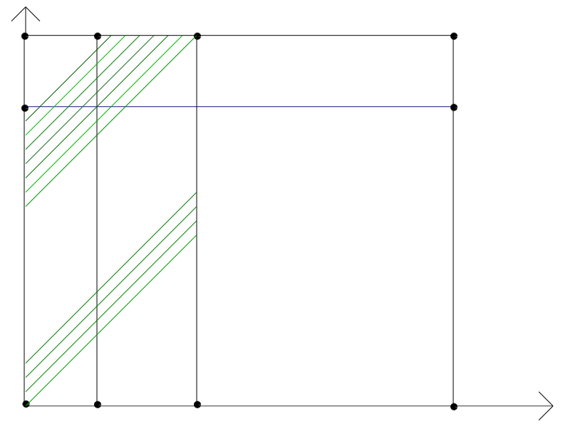
Figure 4. Estimation of n(x,0,t) and l(x,0,t). Here we have chosen a_1=b_1 and a_2=b_2=b..Since t\in (0,T-a_1) all the backward characteristics starting from (0,t) enter the observation domain
We state these two propositions necessary for the proof of the inequality:
Proposition 2.3
Under the assumptions (H_1)-(H3), for all T>\max\{a_1,A-a_2\}, there exists C_T>0 such that the solution (n,l) of the system (2.4) verifies the following inequality:
\int_{0}^{A}\int_{\Omega}n^{2}(x,a,0)dxda\leq C_T\int_{\Xi}n^{2}(x,a,t)dxdadt. (2.14)
Remark 2.2
Note that here we first show that n(x,a,0)=0 in (a_0,A) and we use the same technique as in the Proposition 2 to estimate n(x,a,0) in (0,a_0).
Proposition 2.4
Under the assumptions (H_1)-(H_2) and the hypothesis
b_1 \lt a_0 \lt b and T \gt b_1. There exists C_T>0 such that the solution (n,l) of the system (2.4) verifies the following inequality:
\int_{0}^{a_0}\int_{\Omega}l^{2}(x,a,0)dxda\leq C_T\int_{\Xi'}l^{2}(x,a,t)dxdadt. (2.15)
Let us gives a preliminary results for the proof of the Theorem 2.2 of [1].
Let l=u_1+u_2 where u_1 and u_2 verify
\left\lbrace \begin{array}{ll} -\dfrac{\partial u_1}{\partial t}-\dfrac{\partial u_1}{\partial a}-K_f\Delta u_1+\mu_f(a)u_1=0&\hbox{ in }Q_{A}\times (0,T-\eta) ,\\ u_1(\sigma,a,t)=0&\hbox{ on }\partial\Omega\times (0,A)\times (0,T-\eta),,\\ u_1\left( x,A,t\right) =0&\hbox{ in } \Omega\times (0,T-\eta) \\ u_1\left(x,a,T-\eta\right)=l_{\eta}&\hbox{ in }Q_{A}. \end{array}\right. (2.16)
and
\left\lbrace \begin{array}{ll} -\dfrac{\partial u_2}{\partial t}-\dfrac{\partial u_2}{\partial a}-K_f\Delta u_2+\mu_f(a)u_2=V(x,a,t)&\hbox{ in }Q_{A}\times (0,T-\eta) ,\\ u_2(\sigma,a,t)=0&\hbox{ on }\partial\Omega\times (0,A)\times (0,T-\eta),\\ u_2\left( x,A,t\right) =0&\hbox{ in } \Omega\times (0,T-\eta) \\ u_2\left(x,a,T-\eta\right)=0&\hbox{ in }Q_{A}. \end{array}\right. (2.17)
where the couple (n,l) verifies
\left\lbrace \begin{array}{ll} -n_t-n_a-K_m\Delta n+\mu_m n=0 &\text{ in }Q ,\\ -l_t-l_a-K_f\Delta l+\mu_f l=V(x,a,t)&\text{ in }Q,\\ n(\sigma,a,t)=l(\sigma,a,t)=0&\text{ on }\Sigma, \\ n(x,a,T)=n_T\quad l(x,a,T)=l_T&\text{ in }Q_A,\\ n(x,A,t)=0,\quad l(x,A,t)=0& \text{ in }Q_T.\\ \end{array} \right. (2.18)
(see for instance [1]), with l_{\eta}=l(x,a,T-\eta) in Q_{A} and
V(x,a,t)=\beta(a,p)l(x,0,t)+\beta(a,p)n(x,0,t).
Using Duhamel’s formula we can write
u_2(x,a,t)=\int\limits_{t}^{T-\eta}\mathbb{T}_{t-f}V(x,a,f)df
where \mathbb{T} is the semigroup generated by the operator -K_f\Delta-\dfrac{\partial }{\partial a}+\mu_f(a).
Proof. Proof of the Theorem 2.2
We split the term to be estimated as follows
\int\limits_{0}^{A}\int_{\Omega}l^2(x,a,0)dxda=\int\limits_{0}^{\max\{a_1,b_1\}}\int_{\Omega}l^2(x,a,0)dxda+\int\limits_{\max\{a_1,b_1\}}^{A}\int_{\Omega}l^2(x,a,0)dxda.
As, \max\{a_1,b_1\} \lt b, using the Proposition 2.4 of [1] we obtain the estimate
\int\limits_{0}^{\max\{a_1,b_1\}}\int_{\Omega}l^2(x,a,0)dxda\leq C\int\limits_{0}^{T}\int\limits_{b_1}^{b_2}\int_{\omega}l^2(x,a,t)dxdadt. (2.19)
We are now left with the estimation of
\int\limits_{\max\{a_1,b_1\}}^{A}\int_{\Omega}l^2(x,a,0)dxda.
But since l=u_1+u_2, we must therefore estimate
\int\limits_{\max\{a_1,b_1\}}^{A}\int_{\Omega}u_{1}^{2}(x,a,0)dxda+\int\limits_{\max\{a_1,b_1\}}^{A}\int_{\Omega}u_{2}^{2}(x,a,0)dxda.
We have
\int\limits_{\max\{a_1,b_1\}}^{A}\int_{\Omega}u_{2}^{2}(x,a,0)dxda\leq C_{\eta,T}(A-\max\{a_1,b_1\})\left(\int\limits_{0}^{T-\eta}\int_{\Omega}l^2(x,0,t)dxdt+\int\limits_{0}^{T-\eta}\int_{\Omega}n^2(x,0,t)dxdt\right).
And then, using the Proposition 2.1 of [1], with \eta=\max\{a_1,b_1\}+\delta<T\hbox{, }\delta>0, we obtain
\int\limits_{\max\{a_1,b_1\}}^{A}\int_{\Omega}u_{2}^{2}(x,a,0)dxda\leq C_{\eta,T}\left(\int\limits_{0}^{T}\int\limits_{b_1}^{b_2}\int_{\omega}l^2(x,a,t)dxdadt+\int\limits_{0}^{T}\int\limits_{a_1}^{a_2}\int_{\omega}n^2(x,a,t)dxdadt\right). (2.20)
As,
T>\max\{a_1,b_1\}+\max\{A-a_2,A-b_2\},
we can choose \delta>0 small enough (\delta should also check, \max\{a_1,b_1\} \lt \min\{a_2,b_2\}-\delta)
such that
T>\max\{a_1,b_1\}+\max\{A-a_2,A-b_2\}+2\delta;
therefore
T-(\max\{a_1,b_1\}+\delta)>A-(\min\{a_2,b_2\}-\delta).
Moreover for
a\in (\min\{a_2,b_2\}-\delta,A)
we have
T-(\max\{a_1,b_1\}+\delta)>A-(\min\{a_2,b_2\}-\delta)>A-a.
Then, from the Remark 2.2 of [1]
u_1(x,a,T)=0\hbox{ a.e. }x\in \Omega\hbox{, }a\in(\min\{a_2,b_2\}-\delta),A).
Therefore
\int\limits_{\max\{a_1,b_1\}}^{A}\int_{\Omega}u_{1}^2(x,a,0)dxda=\int\limits_{\max\{a_1,b_1\}}^{\min\{a_2,b_2\}-\delta}\int_{\Omega}u_{1}^{2}(x,a,0)dxda.
As
T-(\max\{a_1,b_1\}+\delta)>A-(\min\{a_2,b_2\}-\delta)),
then using the Proposition 2.3 of [1], we obtain
\int\limits_{\max\{a_1,b_1\}}^{A}\int_{\Omega}u_{1}^{2}(x,a,0)dxda\leq K\int\limits_{0}^{T-\eta}\int\limits_{b_1}^{b_2}\int_{\omega}u_{1}^{2}(x,a,t)dxdadt. (2.21)
As
u_1=l-u_2,
then
\int\limits_{0}^{T-\eta}\int\limits_{b_1}^{b_2}\int_{\omega}u_{1}^{2}(x,a,t)dxdadt
\leq 2\left(\int\limits_{0}^{T-\eta}\int\limits_{b_1}^{b_2}\int_{\omega}u_{2}^{2}dxdadt+\int\limits_{0}^{T-\eta}\int\limits_{b_1}^{b_2}\int_{\omega}l^{2}(x,a,t)dxdadt\right). (2.22)
Moreover, under the assumption of Theorem 1.1 of [1], the solution u_2 of the system (2.22) verifies the following estimate :
\int\limits_{0}^{T-\eta}\int\limits_{b_1}^{b_2}\int_{\omega}u_{2}^2(x,a,t)dxdadt\leq \int\limits_{0}^{T-\eta}\int\limits_{0}^{A}\int_{\Omega}u_{2}^2(x,a,t)dxdadt
\leq C \left(\int\limits_{0}^{T-\eta}\int_{\Omega}l^2(x,0,t)dxdt+\int\limits_{0}^{T-\eta}\int_{\Omega}n^2(x,0,t)dxdt\right). (2.23)
where C=e^{\frac{3}{2}(T-\eta)}\|\beta\|^{2}_{\infty}A.
From the Proposition 2.1 of [1], we get
\int\limits_{\max\{a_1,b_1\}}^{A}\int_{\Omega}u_{1}^{2}(x,a,0)dxda\leq C(T,\eta,\|\beta\|_{\infty})\left(\int\limits_{0}^{T}\int\limits_{b_1}^{b_2}\int_{\omega}l^{2}(x,a,t)dxdadt+\int\limits_{0}^{T}\int\limits_{a_1}^{a_2}\int_{\omega}n^{2}(x,a,t)dxdadt\right). (2.24)
Combining the inequalities (2.23) and (2.24), we obtain
\int\limits_{\max\{a_1,b_1\}}^{A}\int_{\Omega}l^{2}(x,a,0)dxda\leq C(T,\eta,\|\beta\|_{\infty}) \left(\int\limits_{0}^{T}\int\limits_{a_1}^{a_2}\int_{\omega}n^{2}(x,a,t)dxdadt+\int\limits_{0}^{T}\int\limits_{b_1}^{b_2}\int_{\omega}n^{2}(x,a,t)dxdadt\right). (2.25)
Therefore, (2.24) and (2.25) give
\int\limits_{0}^{A}\int_{\Omega}l^{2}(x,a,0)dxda\leq K_{T} \left(\int\limits_{0}^{T}\int\limits_{a_1}^{a_2}\int_{\omega}n^{2}(x,a,t)dxdadt+\int\limits_{0}^{T}\int\limits_{b_1}^{b_2}\int_{\omega}n^{2}(x,a,t)dxdadt\right). (2.26)
Finally, combining (2.26) and the inequality of the Proposition 2.3 of [1], we get the observability inequality.
Illustration of the observability inequality and estimation of the non local terms
Let \Lambda be a operator define as follow:
\Lambda: L^{2}(Q_T)\longrightarrow L^{2}(Q_T)\quad p\longmapsto \int_{0}^{A}\lambda (a)m(p)da (2.27)
where the couple (m(p),f(p)) is the solution of the following auxilliary system verifying
m(x,a,T)=0 \hbox{ a.e. } x\in \Omega \hbox{ } a\in (0,A), (2.28)
f(x,a,T)=0 \hbox{ a.e. } x\in \Omega\hbox{ } a\in (0,A). (2.29)
Under the assumptions of Theorem 1.1, we can show that the operator \Lambda is continuous, and the set \Lambda(L^{2}(Q_T)) is relatively compact in L^{2}(Q_T).
By Schauder’s fixed point theorem \Lambda admits a fixed point and we get the reult of the Theorem 1.1. Let us gives a preliminary results for the proof of the Theorem 3.1. of [1].
We denote by
Q=\Omega\times (0,A)\times (0,T)\hbox{, }Q_A=\Omega\times(0,A)\hbox{, }Q_T=\Omega\times (0,T)\hbox{ and }\Sigma=\partial\Omega\times (0,A)\times (0,T). \square
Numerics Simulations without the space variable
We start with a mesh of segment [0,A]. By the method of finite differences we get,
\dfrac{\partial m}{\partial a}(a_j,t)=\dfrac{m(a_{j},t)-m(a_{j-1},t)}{\Delta a},
\dfrac{\partial f}{\partial a}(a_j,t)=\dfrac{f(a_{j},t)-f(a_{j-1},t)}{\Delta a},
which corresponds to the approximation of the aging terms at the different points of the mesh. Let m_{j}(t) and f_{j}(t) the approximation of m(a_j,t), f(a_j,t) and U_{l}(t) = (m_{j}(t),f_{i}(t))_{1\leq j\leq N ,\quad 1\leq i\leq N}, and Y_l=(y(a_i))_{1\leq i\leq N} the initial condition vector and A_l the matrix of the mortality approximation and the aging approximation.
So we get the following system
\dot{U_l}=A_lU_l+\text{vectorF}+BV_l\text{ with }U_l(0)=Y_l
where B is a matrix defining the control support of the matrices, vectorF is the contribution of the nonlocal part, which comes from the births and V_l(t) the control vector which also comes from the nonlocal term.
Using matlab’s ODE 45 we obtain the following results:
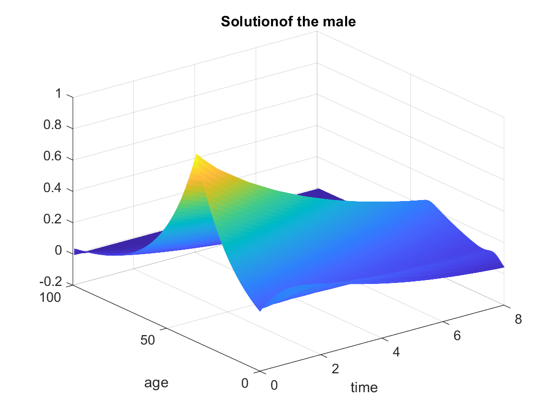
Figure 5. Solution of the male
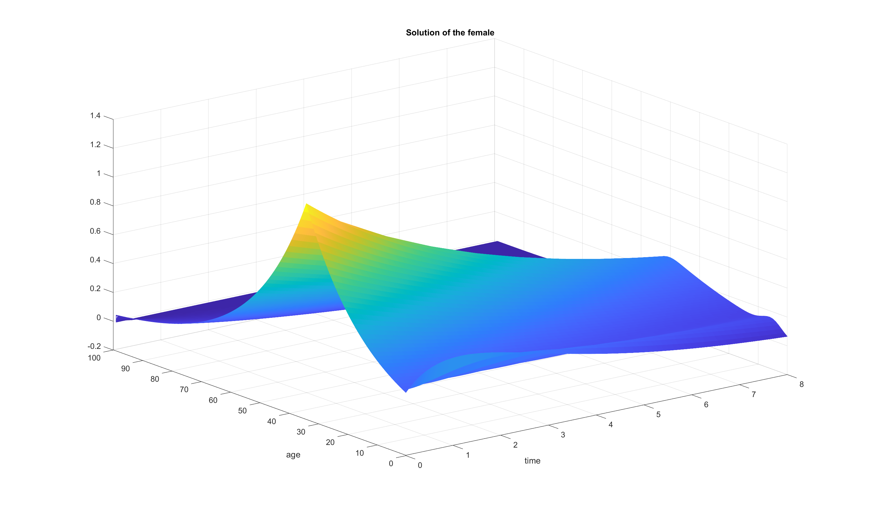
Figure 6. Solution of the female.
For the approximate null controllability we minimize the functional
J_\epsilon(V_l)=\dfrac{1}{\epsilon}\int\limits_{0}^{A}|U_l(T)|^2+\int\limits_{0}^{T}\int\limits_{0}^{A}|V_l(t)|^2dadt
under the constraint
\dot{U_l}=A_lU_l+\text{vectorF}+BV_l\text{ et }U_l(0)=(m_{00},f_{00}).
Using Casadi’s algorithm, we can see the following result:
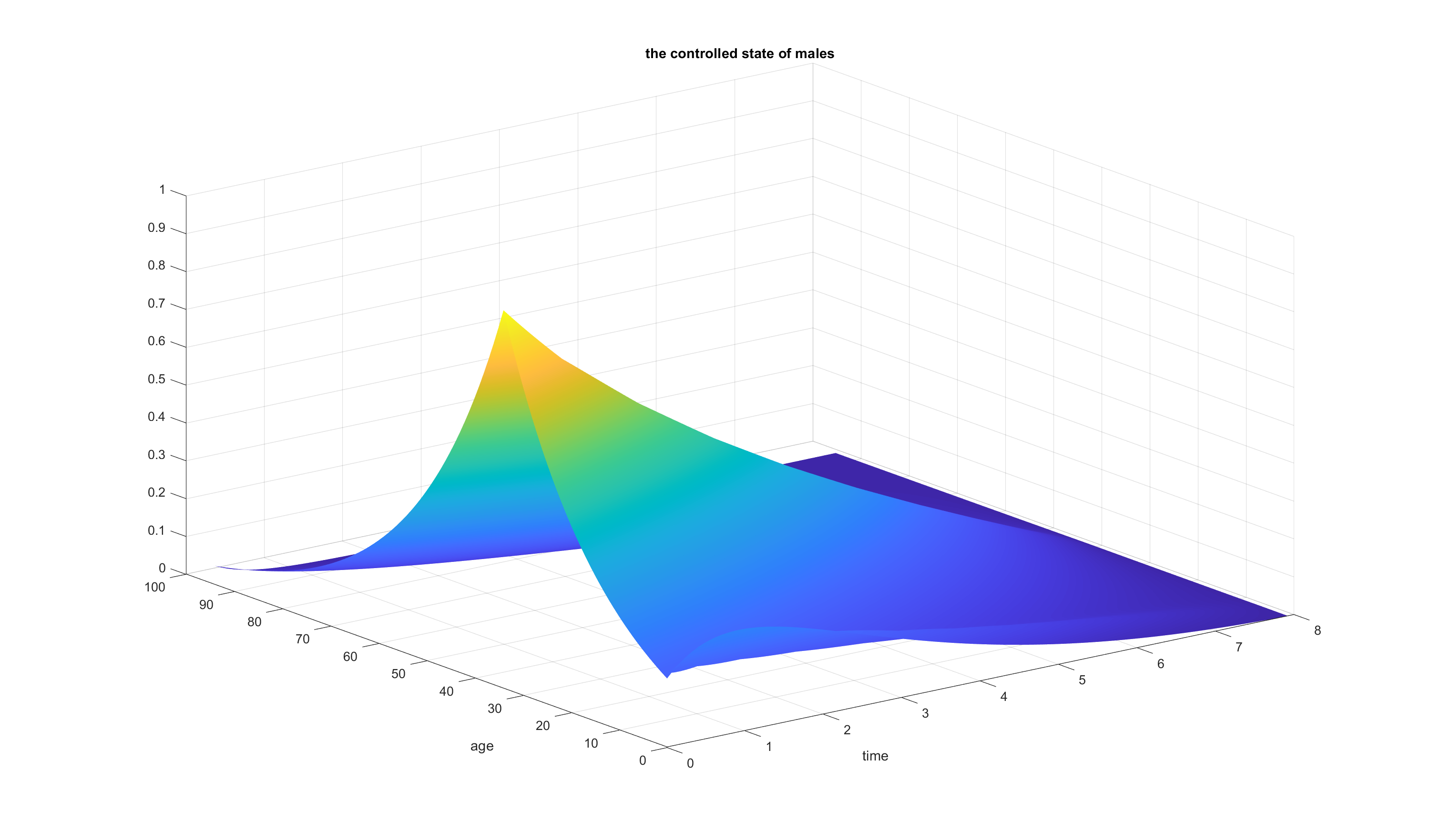
Figure 7. Solution of the male
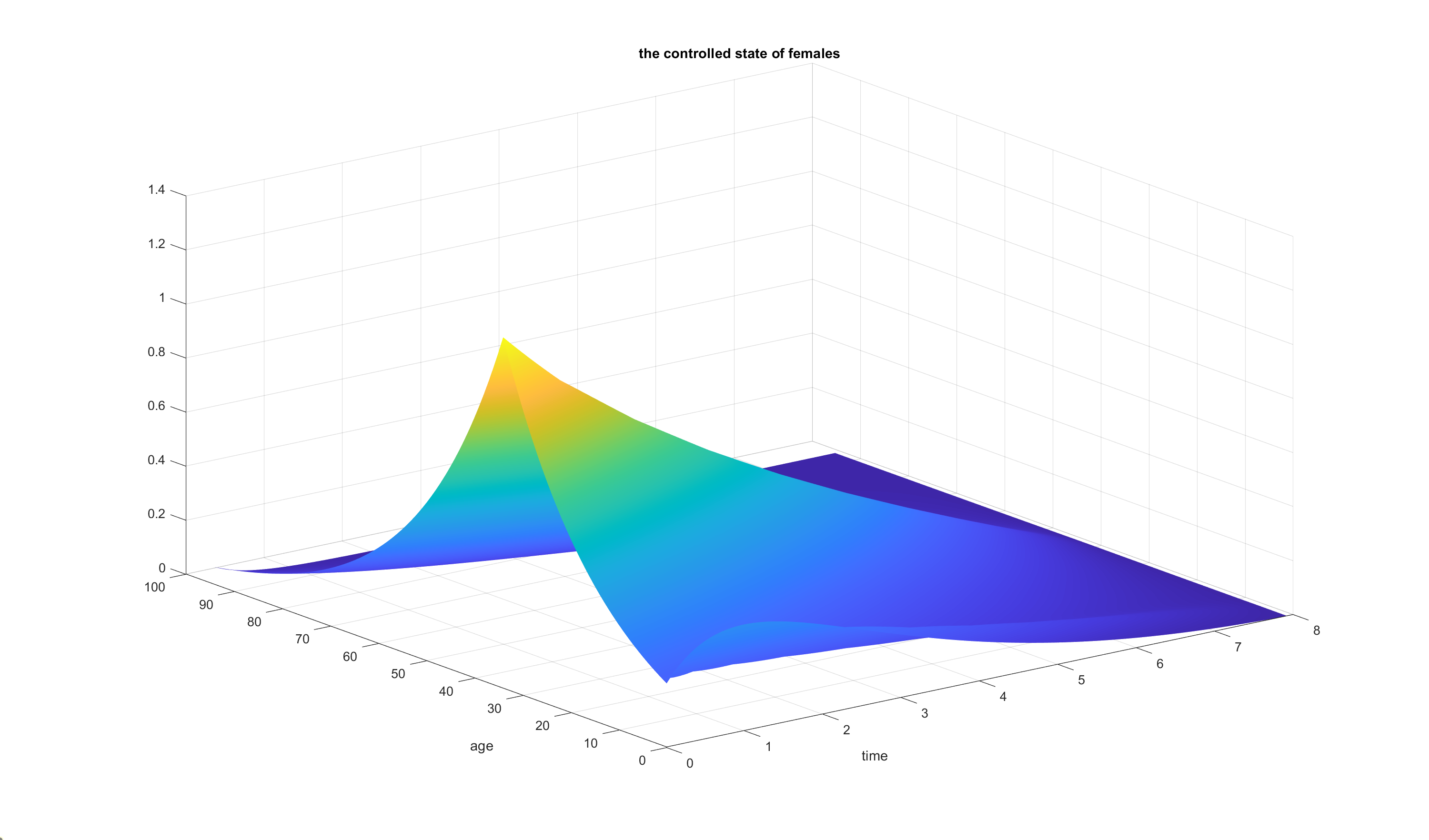
Figure 8. Solution of the female.