Long-time behavior of locally and partially dissipated hyperbolic systems

Spain 26.07.2022

Long-time behavior of locally and partially dissipated hyperbolic systems

Author: Timothée Crin-Barat

In this post we are interested in the long-time behavior of solutions to locally and partially dissipated hyperbolic systems. Our goal is to recover the decay rates from the classical case modulo some delay depending on the size of the undamped regions and the eigenvalues of the system.
But first, we take a step back and provide a quick introduction on partially dissipative systems.
 

1 Partially dissipative hyperbolic systems

1.1 Basic presentation

In the context of these notes, by partially dissipative system we refer to systems of $n$ equations such that dissipative mechanisms (as e.g. friction or drag forces) are only active in $n_2$ equations with $n_2 \lt n$. This definition is in contrast with the stronger totally dissipative condition, for which $n_2=n$, ensuring that all the components are exponentially damped. Even if it leads to better, asymptotically speaking, results the latter condition is not very natural for physical real-world applications. For instance, when modelling a compressible fluid, it is not physically-relevant to consider dissipative mechanism acting directly in the equation of the density of the fluid as it usually satisfy a conservation law. On the other hand, the partially dissipative condition is much more reasonable as it is satisfied by a large number of systems modelling real-world phenomena, but, as we will see, issues of high complexity arise from it.
 
Let us have a look at the simplest ODE settings first. In this context, such systems of $n$ equations read

$∂_t U(t) + BU(t)=0  (1)$

where $U=(u_1,\ldots,u_n)$ and $B=\begin{pmatrix}0 & 0 \\ 0 & D \end{pmatrix}$ with $D$ a positive definite $n_2 \times n_2$ matrix such that $n=n_1+n_2$.
Developing the compact form of the system, we can rewrite it as

$\begin{cases} & ∂_t u_1 =0 \\ \qquad\vdots \\& ∂_t u_{n_2-1}=0 \end{cases} \text{and} \begin{cases} & ∂_t u_{n_2} +u_{n_2}=0 \\\qquad\quad\vdots \\& ∂_t u_{n} +u_{n}=0. \end{cases}$

Above the 0-th order terms correspond to dissipative effects and allows to justify exponential decays for the components $u_i$ with $n_2\leq i\leq n.$ For the other components one can only say that there are constants that can be determined by the initial data.

In the previous example, the partially dissipative condition is not so mysterious, but if one considers the system:

$∂_t U(t)+AU(t)+BX(t)=0$

where $X$ is the control, then it is known that the Kalman rank condition for the couple $(A,B)$ implies its controllability in time $T>0$.
And it is possible to find a feedback control such that the solution have exponential decay. In a sense, for a given matrix $A$, the Kalman condition allows you to test whether adding to $A$ a given matrix $B$ lead to the desired decay rates or not. But it does not tell you specifically what $B$ should look like.

 

Remark 1.1.

Note that even in the context of ODE’s, the Kalman condition raise questions of very high complexity. For instance: for a given matrix $A$ which matrix B such that $(A,B)$ satisfy the Kalman condition leads to the best decay rates? Or, what is the minimum number of controlled equations that one needs to ensure the controllability of the system? And many other problems which, of course, are transposed to the world of PDEs, sometimes in an even trickier manner.

Related to these considerations, recent development have been made in the context of PDE’s and this is what we shall discuss below.
More precisely, we will see how “adding” a hyperbolic structure, that on its own is conservative, to a partially dissipated system can modify the behavior of the solution drastically.
 

1.2. Partially dissipative hyperbolic systems

In the context of PDE’s we look at the following hyperbolic partially dissipative systems in the one-dimensional setting:

$∂_t U +A ∂_x U+ BU=0  (2)$

where $A$ is a symmetric matrix and the others terms are defined as previously. The symmetric assumption is there to ensure that the system under study is hyperbolic and therefore locally well-posed i.e. one can ensure the existence of local-in-time solutions. Concerning the global well-posedness, it depends on the interaction between the matrices $A$ and $B$, as we will see below.

These systems model physical phenomena with finite speed of propagation or equilibrium laws, such as the compressible Euler equation with damping:

$\displaystyle\left\{\displaystyle \begin{matrix} ∂_t\rho+ div(\rho u)=0,\\[1ex]\displaystyle ∂_t u +u \cdot \nabla u +\nabla P(\rho)+u=0. \end{matrix} \right.  (3)$

In contrast to the previous situation, even if the dissipative mechanism is only present in some of the equations, we will see that it is possible, under certain reasonable conditions, to recover dissipation for all the components of the system. Essentially, this is made possible by looking at the interaction between the hyperbolic part and the dissipative part of the system.
Let us see how this can be achieved in a simple case.

 
1.2.1. Study of a toy-model
The canonical toy-model for such problems is the following system:

$\left\{ \begin{matrix}\partial_tu+ ∂_xv=0,\\[1ex] \partial_tv+ ∂_xu+ \textcolor{red}{v}=0, \end{matrix} \right.  (4)$

where the red term corresponds to the partial dissipation. Performing standard energy estimates, one obtains

$\frac{d}{dt}\|(u,v)\|+\|v\|_{L^2}^2\leq 0)  (5)$

which shows a lack of coercivity for the unknown $u$ and does not allow to conclude time-decay property for both unknowns.

Idea: consider the following perturbed functional

$\mathcal{L}^2=\|(u,v, ∂_xu, ∂_xv)\|_{L^2}^2+\textcolor{blue}{\int_\mathbb{R}v ∂_xu}.$

Differentiating in time this functional allows to justify decay estimates for both components.
Indeed, one easily obtains

$\frac{d}{dt}\mathcal{L}^2+\|v\|_{L^2}^2+\|(\textcolor{blue}{ ∂_xu}, ∂_xv)\|_{L^2}^2\leq 0$

which now also highlights some time-decay properties for $u$.

From here, one can conclude decay-estimates using that $\mathcal{L}^2\sim \|(u,v, ∂_xu, ∂_xv)\|_{L^2}^2$, however, due the special structure of the previous inequality, one cannot conclude exponential decay uniformly in frequency.
For a given initial data $U_0=(u_{1,0},u_{2,0})\in L^1\cap L^2$, one obtains

$\|U^h(t)\|_{L^2(\R^d,\R^n)}\leq Ce^{-\lambda t}\|U_0\|_{L^2(\R^d,\R^n)},$

$\|U^\ell(t)\|_{L^\infty(\R^d,\R^n)}\leq Ct^{-\frac{d}{2}}\|U_0\|_{L^1(\R^d,\R^n)}$

where $U^h$ and $U^\ell$ correspond, respectively, to the high and low frequencies of the solution.
Such frequency decomposition is unavoidable as the behavior in both regime is fundamentally different. Such behavior can actually be anticipated by a spectral analysis of the system which depict it exactly.

 

Remark 1.2.

A more precise decomposition can actually be obtained following recent development in [4] where a purely damped mode was highlighted in the low frequency setting. In particular, it implies that one can improve the low-frequency decay rates.

 
1.2.2. Back to the general system
We have just seen how, on a simple partially dissipative model, we can recover the dissipation for all unknowns, at the cost of lower decay rates.
Let us now see how to generalize this analysis to general partially dissipative hyperbolic systems (2).

To overcome the lack of coercivity, Shizuta and Kawashima in [9] developed a condition, the well-known stability condition (SK), which ensures the decay of our solution to $0$ when $t\to\infty$:

$(SK)   \{\text{eigenvectors of } A \xi\} \cap \mathrm{Ker}(B) = \{0\}, \quad \forall\xi \in \R^*.$

In one space dimension, this condition is equivalent to the fact that there are no plane wave solutions to the hyperbolic system propagating to the characteristic directions and therefore ensures the decay of our solutions; in higher dimensions, it is known that the (SK) condition is sufficient to ensure such properties but not necessary.

Moreover, this condition is actually equivalent to the Kalman rank condition for all the pairs $(A\xi,B)$ with $\xi\ne0$. Inspired by this and the hypercoercivity theory introduced by Villani, Beauchard and Zuazua in [1] defined the following generalized Lyapunov:

$\mathcal{L}^2\triangleq \|V\|_{L^2}^2 + \int_{\R^d} \min(\rho,\rho^{-1})\mathcal{I} \quad\text{where}\quad \mathcal{I}\triangleq \Im \sum_{k=1}^{n-1} \varepsilon_k \bigl(LA_\omega^{k-1}\widehat{V} \cdot LA_\omega^k \widehat{V} \bigr)$

where $\xi=\rho \omega$. This time, using the (SK) condition and choosing correctly the constants $\varepsilon_k$, after few pages of computations one obtains

$\frac d{dt}\mathcal{L} +\kappa \min(1,|\xi|^2) \mathcal{L} \leq 0.$

And from here, we can get the same decay rates as before. Let us mention that it was proven in [1] that in the one-dimensional context, the condition $(SK)$ is equivalent to the fact that:
• In low frequencies, the solution behaves as the solution of the heat equation
• In high frequencies, the solution decays exponentially.

 

Remark 1.3.

In higher dimensions, the (SK) condition is actually not necessary to justify the decay rates of such systems. For more details about this, we refer to [1].

More can be said concerning the global well-posedness, asymptotic and relaxation of quasilinear (i.e. $A=A(U)$) hyperbolic partially dissipative systems but this is not the main purpose of this note and we refer to [4, 3, 2] for more details.

 

2. Localized dissipation

 

2.1. Presentation of the problem

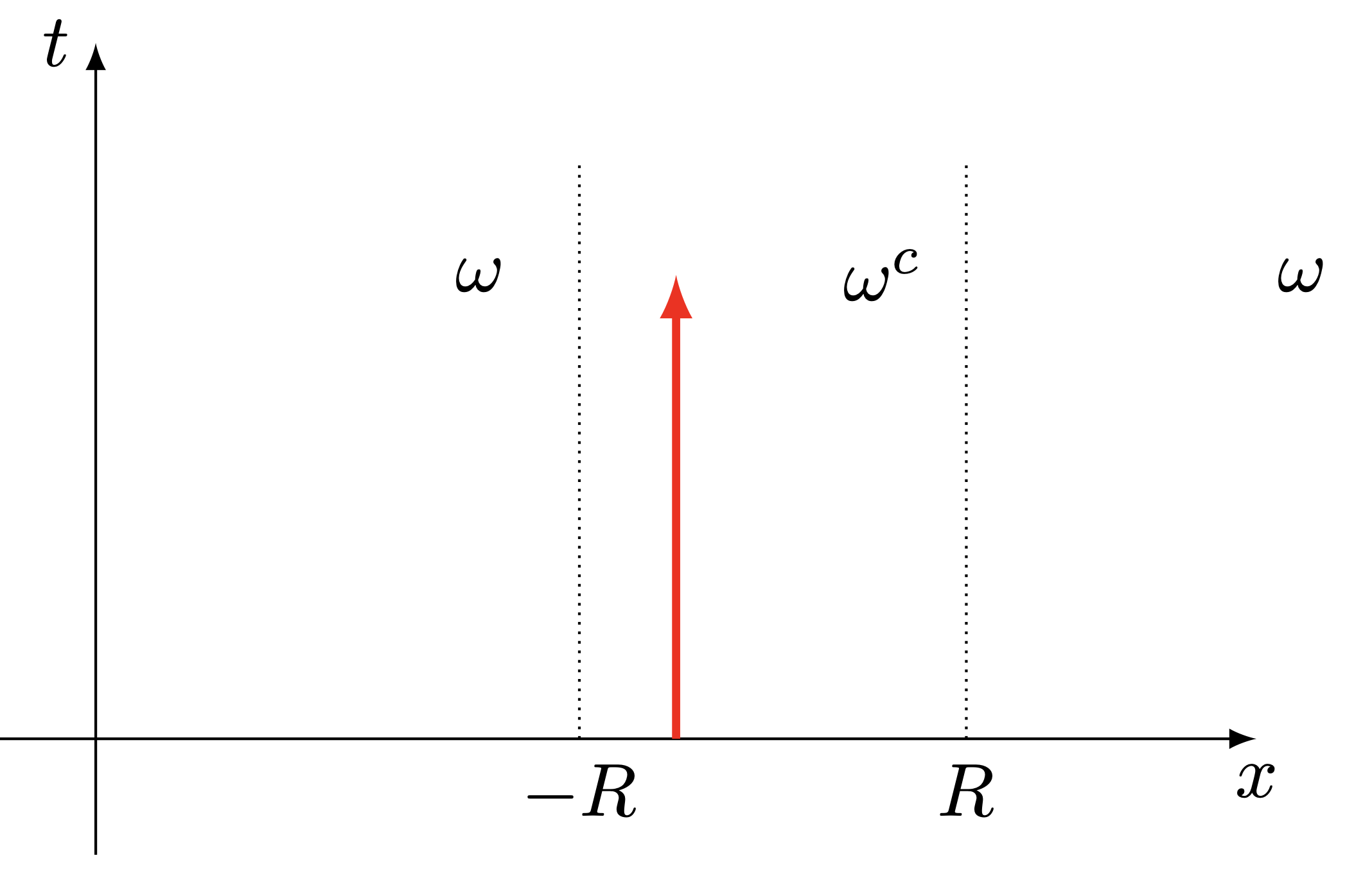
We now turn to the central part of these notes: the case where the damping is only active outside a ball.

This scenario can be represented by the following system:

$\begin{cases} ∂_t U + A ∂_x U = -B U {\color{blue}{\boldsymbol{1}_\omega}}, & (t,x) \in (0,\infty) \times \R, \\ U(0,x) = U_0(x), & x \in \R, \end{cases}  (6)$

where $U = (u_1,u_2) \in \R^{n_1}\times \R^{n_2}$ and

$\textcolor{blue}{ \omega := \R \setminus B_R(0) = \{x \in \R: \| x \| \ge R \} \quad \text{ for a fixed R >0 } }.$

We assume:
• $B=\begin{pmatrix}0&0\\0&D \end{pmatrix}$ with $D>0$ .
• The matrix $A$ is a \emph{strictly hyperbolic matrix}, i.e. $A$ has $n$ real distinct eigenvalues

$\lambda_1 \lt \lambda_p \lt 0 \lt \lambda_{p+1} \lt \lambda_{n}.$

• The couple $(A,B)$ satisfies the (SK) condition.

In other words: we are in the same situation as before but the damping is only effective in $\omega$ (the complementary of a ball).

  Goal: Quantify the decay as in the classical case.

Difficulties:
• The approach depicted previously is bound to fail as it relies on the Fourier transform. Indeed, applying the Fourier transform in this setting would lead to convolution operation that we do not know how to extract information from.
• Defining a perturbed functional is not enough to solve this problem, as it is known for the damped wave equations.

 
Idea:
• The characteristic lines of the system spend only a finite time in the undamped region.
• When a characteristic is outside the undamped region, the solution decays as in the classical analysis.

$\rightarrow$ This motivates us to develop a method involving only the consideration of the characteristics curves and a semigroup-wise decomposition.

 

2.2. Presentation of the method to get decay rates

Let us see how the characteristics propagate depending on their location with respect to the region $\omega = \R \setminus B_R$ (where the damping is active). This is depicted in the following figure

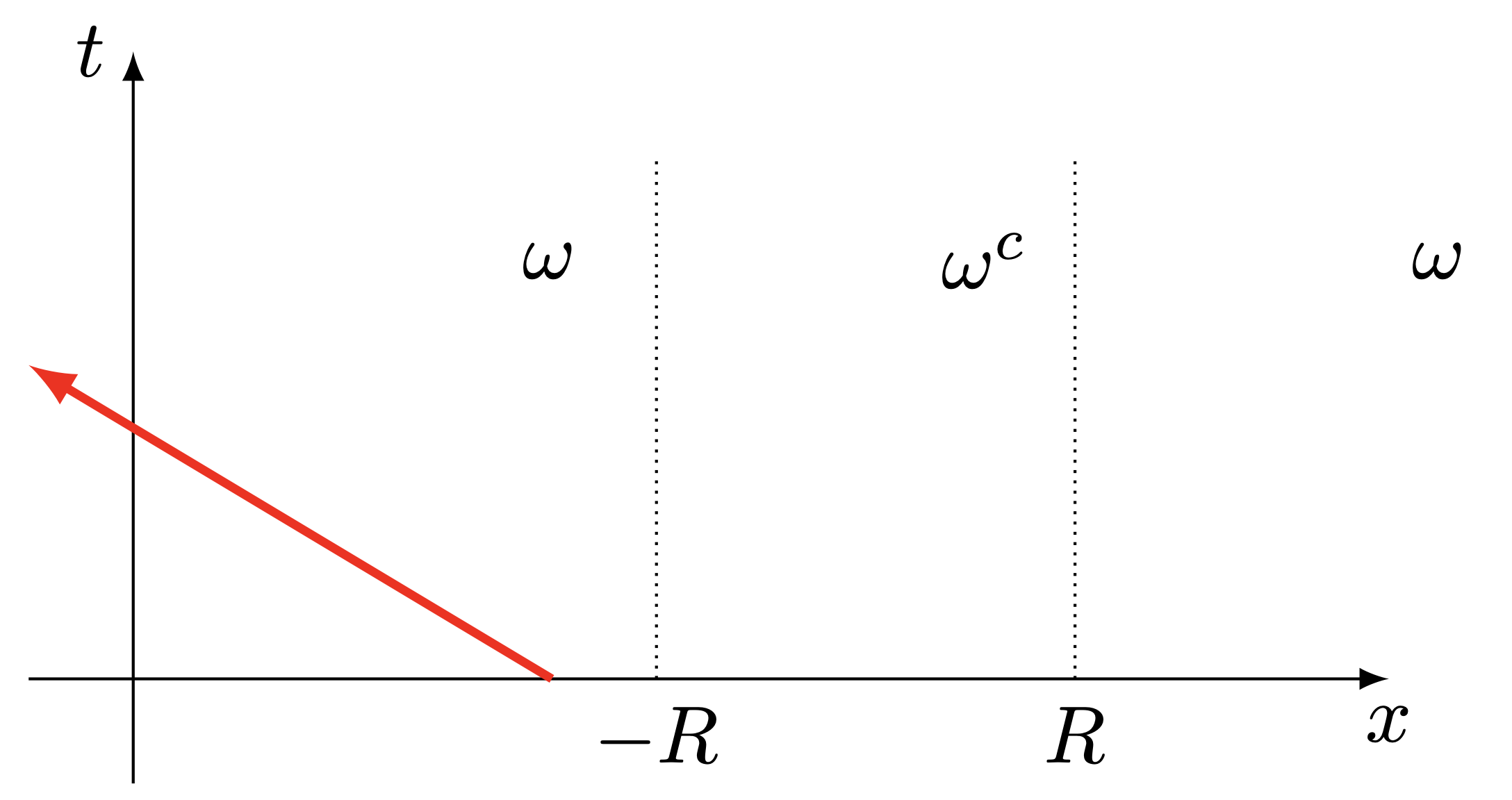
(a)Case 1. The initial support is in the damped region and the characteristics are going away from the un-damped region.

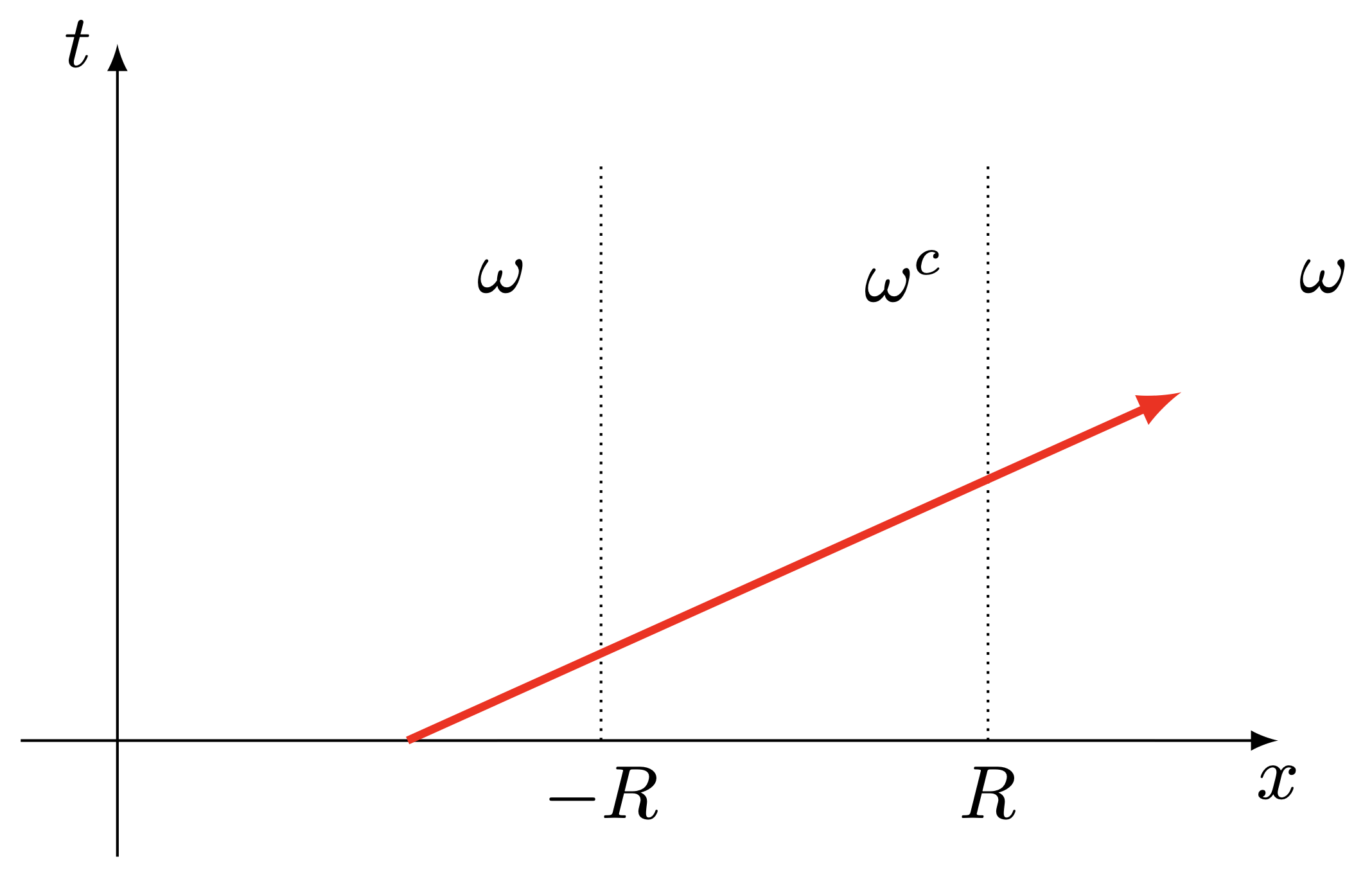
(b)Case 2. The initial support is in the damped region and the characteristics cross the un-damped region

(c)Case 3. The initial support is in the un-damped region

(d)Case 4. There is one zero eigenvalue. $\rightarrow$ Standing wave

From this figure, we deduce one crucial fact: when there are no 0-eigenvalues, the characteristics only spend a finite time in the undamped region. And thus one expects to recover similar asymptotic as in the previous case for large times. But, concretely speaking, how can we use this to justify the desired decay?

First, one should reformulate the system to highlight the transport part in each equations.

 
2.2.1. Reformulation of the system
Our reformulation is based on the diagonalisation of the matrix $A$. As $A$ is symmetric with $n$ real distinct eigenvalues, there exists a matrix $P \in O(n,\mathbb{R})$ such that

$P^{-1}AP=\Lambda \quad \text{where} \quad \Lambda=\operatorname{diag}(\lambda_1,...,\lambda_n).$

Setting $V=P^{-1}U$, the system can be reformulated into

$\begin{cases} ∂_t V + \Lambda ∂_x V = P^{-1}BPV \boldsymbol{1}_\omega(x), & (t,x) \in (0,\infty) \times \R, \\ V(0,x) = V_0(x), & x \in \R, \end{cases}  (7)$

 

Remark 2.1.

We remark that, as the (SK) condition is satisfied, if $A$ and $B$ commute, we can diagonalize the matrices simultaneously and the problem ends up to be totally decoupled and related to the totally dissipative case.

Decomposing $V=(v_1,\ldots,v_n)$, System (7) is equivalent to the following system of coupled transport equations:

$\begin{cases} ∂_t v_1 +\lambda_1 \partial_xv_1 &=\sum_{j=1}^nb_{1,j}v_j\,\boldsymbol{1}_\omega(x) \\ &\:\vdots\\ ∂_t v_n +\lambda_n \partial_xv_n &=\sum_{j=1}^nb_{n,j}v_j\,\boldsymbol{1}_\omega(x). \end{cases}$

For this system, for all $1\leq i\leq n$, the characteristic lines $X_i$ of each equations passing through the point $\left(x_{0},t_{0}\right) \in \mathbb{R}\times [0, T]$ are given by

$X_i\left(t, x_{0}, t_{0}\right) := \lambda_i(t-t_{0})+x_{0}, \quad t \in[0, T]$

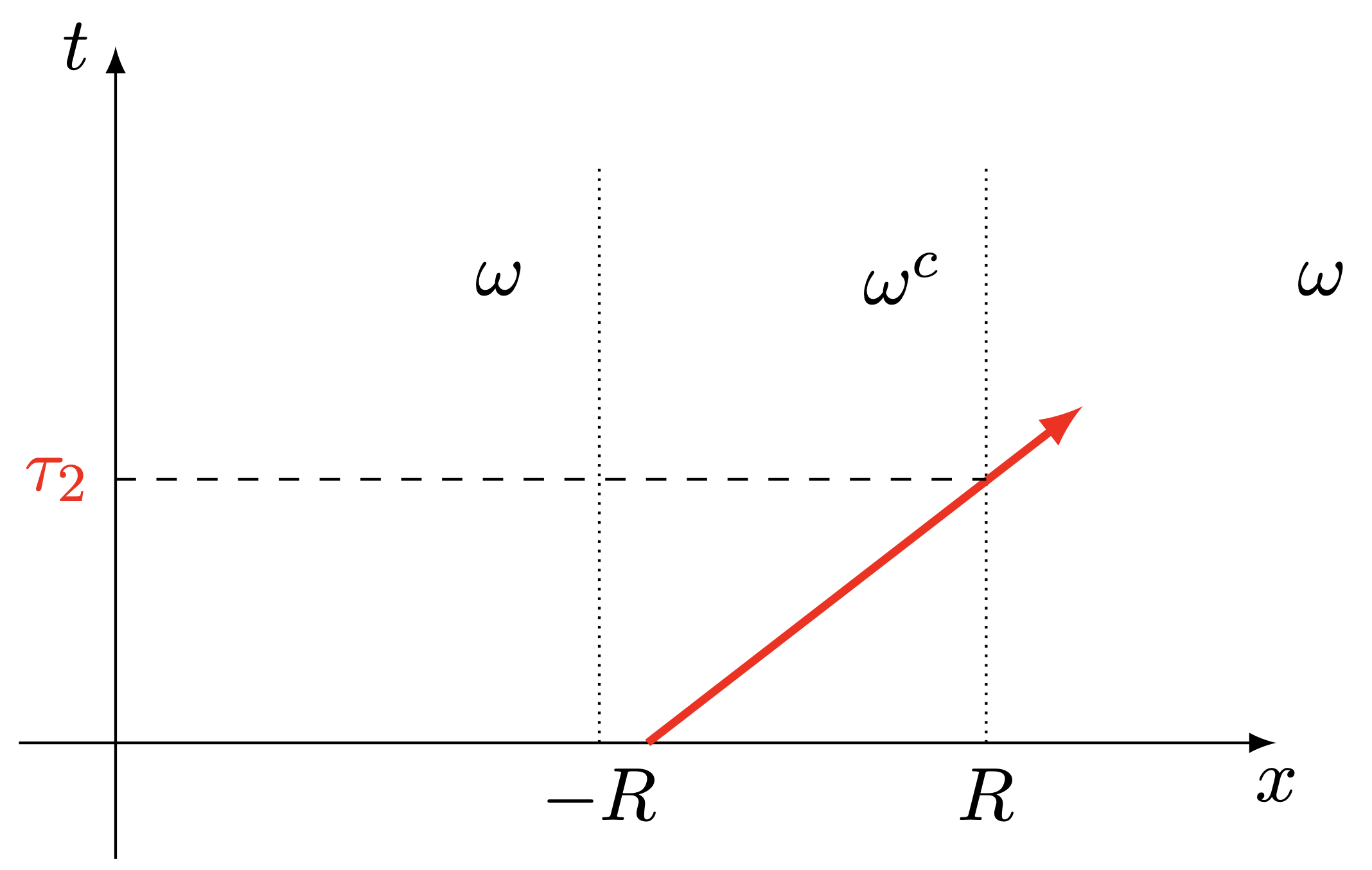
and are depicted in the following figure.

 

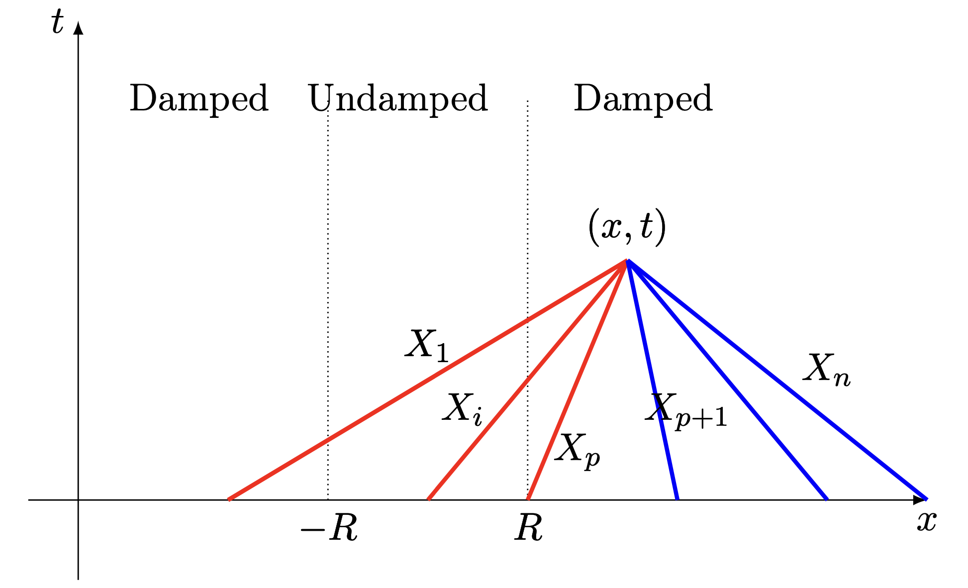
Figure 1. Characteristics passing through a point $(x,t)$.
 

For instance, the damped wave equation $∂_{tt} u - ∂_{xx}^2 u + ∂_t u = 0$ can be rewritten as

$\begin{cases} ∂_t p - ∂_x p = -\frac{1}{2} (p+r)\boldsymbol{1}_\omega,\\ ∂_t r + ∂_x r = -\frac{1}{2} (p+r)\boldsymbol{1}_\omega. \end{cases}$

2.2.2. Remarks and formal analysis leading to the main theorem

As one can see, once a characteristic has crossed and exited the undamped region $\omega^c$ it will never cross it again and the time spent by each characteristics $\tau_i$ in $\omega^c$ satisfies:

$\tau_i\leq \frac{2R}{\lambda_i}.$

This is linked to our choice of $\omega$ as exterior domain which is motivated by a geometric control condition: the ray of geometric optics may escape the damping effect if the inclusion $\{\| x \| \ge r\} \subset \omega$ is not satisfied for some $r>0$.

From here, we may anticipate the desired result by following two principles:
1. The total time spend by all the characteristics in the undamped region is finite.
2. Whenever one of the characteristic is in the undamped region, then the solution does not, in general, undergo any decay.

• The first point is a direct consequence of the previous geometric analysis of the characteristics.
• The second principle, is less direct. As seen in the first section of this notes, since our system has a partially dissipative nature, it is only possible to recover dissipation for all the variable via the coupling between the each equations. And therefore, when one of the characteristics is in the undamped region, one of the coupling term vanish and, in general, this may breaks the dissipative mechanism for all the components.

 

Remark 2.2.

It may happen that the dissipation does not arise from the coupling between each equations. Indeed, considering two decoupled partially dissipative system each verifying (SK), the union of both also verify (SK) but there are no interactions between each systems. Therefore, in practice some components may decays faster than others. but here we focus on the general scenario.

Combining all these considerations led us to the following theorem.

 

Theorem 2.1.

(T. Crin-Barat, N. De Nitti and E. Zuazua ’22)
Assume that the matrix $A$ is symmetric, strictly hyperbolic and does not admit the eigenvalue 0, and that the couple $(A,B)$ satisfies the (SK) condition. Let $U_0\in L^1(\R)\cap L^2(\mathbb{R})$.

Then, there exists a constant $C>0$ and a finite time $\bar{\tau}>0$ such that for $t\geq\bar{\tau}$, the solution satisfies

$\| U^h(\cdot,t) \|_{L^2(\R)} \le Ce^{-\gamma (t-\bar{\tau})} \| U_0 \|_{L^2(\R)}, \\ \| U^\ell(\cdot, t) \|_{L^\infty(\R)} \le C (t-\bar{\tau})^{-1/2} \| U_0 \|_{L^1(\R)}$

where

$\displaystyle\bar{\tau}=\max\left(\sum_{i=1}^p\dfrac{2R}{|\lambda_i|},\sum_{i=p+1}^n\dfrac{2R}{|\lambda_i|}\right).$

In other words, this theorem states that: the classical decay estimates are delayed by the time each characteristic spend in the undamped region. And this delay also depends on whether it is the characteristics going to the left or to the right that spend more time in the undamped region.

 

Remark 2.3.

In the exponential decay inequality, it seems that there are too many constants in the sense that if we set $C'=Ce^{\gamma\bar{\tau}}$ then one could have a more compact form. Here, we prefer the two-constant form because we are able to provide an explicit formula for the delay perceived by the time-decay rates of the energy, and $C$ refers to the same constant as in the classical decay case.

Let us now give more details about the proof of this theorem.
 

2.3. Idea of proof

 
Our method relies on the description of the solution of (6) employing the characteristic method and by distinguishing whether we are in the undamped region or not.
 
To that matter we denote $S_d$ the dissipative semigroup associated to the equation without localization i.e. ($\omega=\R)$. This semigroup is active when all the characteristics are outside the undamped region. It corresponds to the classical decay rates, recall that we have

$\|S_d^h(t,0) U_0^h \|_{L^2(\R^d)} \le C e^{-\gamma t} \| U_0^h \|_{L^2(\R^d)}, \\ \|S_d^\ell(t,0) U_0^\ell \|_{L^\infty(\R^d)}\le C t^{-d/2} \| U_0^\ell \|_{L^1(\R^d)}.$

We denote $S_c$ the conservative semigroup associated to the equation without dissipation at all i.e. ($\omega=\emptyset)$. Essentially, this semigroup will be “dominant” whenever one of the characteristic is inside the undamped region. We have

$\|S_c(t,0)U_0\|_{L^p(\R)}=\|U_0\|_{L^p(\R)}.$

Then, for every $(x,t)\in \R^2$, we can always find suitable times $t_1,t_2$ such that each components of the solution can be rewritten:

$\color{blue} v_i(x,t)=S_{d,i}(t)S_{c,i}(t_1)S_{d,i}(t_2)v_{i,0}(x),  (8)$

where $S_{d,i}$ and $S_{c,i}$ are the semigroup associated to each components i.e. $S_d=(S_{d,1},\cdots,S_{d,n})$ and similarly for $S_c$.

The following figure helps to understand the definition of the semigroups.

 

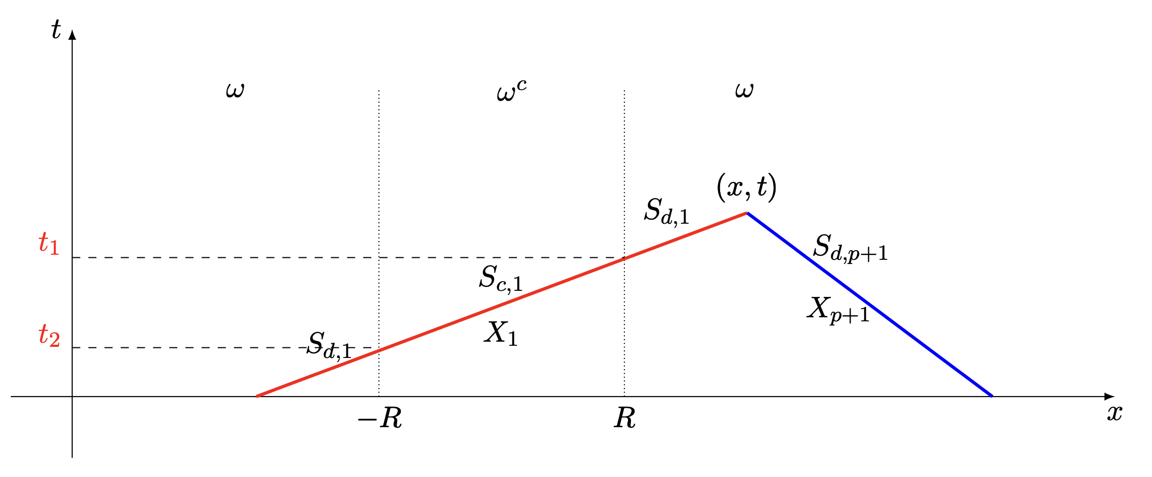
Figure 2. Illustration on the semigroups and the quantities $t_1$ and $t_2$.

One difficulty arising from this representation of the solution comes from that the time-quantities $t_1$ and $t_2$ depend on the point $(x,t)$ as one can easily see on the previous figure. But, essentially, this will be handled by the fact that the difference $t_1-t_2$ is always uniformly bounded.

2.3.1. Difficulties due to partial dissipation
Here we list some of the difficulties that arise due to the partial dissipation context. Note that in the case of totally dissipative systems, the analysis below can be simplified a lot cf. [7].

• It is only possible to obtain dissipation for the solution $V$ if all the semigroups $S_{d,i}$ are active on a same time-interval i.e. the “full” semigroup $S_d=(S_{d,1},\cdots,S_{d,p})$ needs to be active.
• For instance, the action of $S_{d,1}$ on the first component does not, in general, imply any time-decay properties for the component $v_1.$

• This means that if one of the conservative semigroups $S_{c,i}$ is active on a time-interval then the whole solution does not experience any decay on this time-interval;
• Of course, it is possible that some components decay “on their own”. But in general the whole solution does not decay.
• Still, when one semigroups $S_{d,i}$ is active, the $L^p$ norms of the solutions stay bounded thanks to the positive semidefiniteness of $B.$

 
2.3.2. Idea of proof

Recalling that $\forall i\in[1,p]$

$v_i(x,t)=S_{d,i}(t)S_{c,i}(t_1)S_{d,i}(t_2)v_{i,0}(x).$

Taking into account the previous considerations, one ends up studying:

$\mathcal{I}(x,t)=\bigcup_{i=1}^p[t_{1,i}(x,t),t_{2,i}(x,t)]  (9)$

which corresponds to the union of time-interval where the dissipation is not active. In other words, $|\mathcal{I}|$ quantifies exactly the delay appearing in the decay rates of the solution.
 
From here, our theorem derives from the fact that

$\sup_{x\geq R,t>0}|\mathcal{I}(x,t)|\leq \displaystyle\sum_{i=1}^p\dfrac{2R}{|\lambda_i|}=\bar{\tau}  (10)$

and computations of the following type:

$\|v_1(.,t)\|_{L^2(\R)} = \|S_{d,1}(t)S_{c,1}(t_{1})S_{d,1}(t_{2})v_{1,0}\|_{L^2(\mathbb{R})} \\$

$\leq e^{-c(t-t_{1})}\|S_{c,1}(t_{1})S_{d,1}(t_{2})v_{1,0}\|_{L^2} \\$

$\leq e^{-c(t-t_{1})}\|S_{d,1}(t_2)v_{1,0}\|_{L^2} \\$

$\leq e^{-c(t-t_{1})}e^{-c(t_{2}-0)}\|v_{1,0}\|_{L^2} \\$

$\leq e^{-c(t-(t_1-t_2))}\|v_{1,0}\|_{L^2}.$

However, we warn the reader that the above computations are not so simple to realize in practice as the time-quantities appearing above should also depend on the space variable. To solve this issue, one needs to use that in this linear setting we may decompose the space-interval into smaller interval, apply the superposition principle and use that $t_1(x)-t_2(x)$ is uniformly bounded.
For more details of these computations we refer to Section 4 of [5].

 

3. Further analysis and extensions

 

3.1. Behavior for smaller times

The estimates (10) for the time-interval $\mathcal{I}$ is sharp for times larger than $\bar{\tau}$ but it can be refined for shorter times. Indeed, for shorter times the previous analysis stays correct but one must consider the fact that the different characteristics may overlap in the undamped region and therefore reduce the delay observed in the decay rates of Theorem 2.1. However, obtaining an optimal bound for $|\mathcal{I}|$ turns out to be very difficult. For more information about this we refer to [5] where we perform a complete analysis in the case of three components.

 

3.2. More general undamped domain

Results similar to ours can be obtained whenever $\omega^c$ is a domain of finite measure. For example, let us consider $\omega^c$ as a finite union of bounded stripes; in this case, we can directly retrieve similar decay estimates with a delay depending on the time spent by each characteristics in each stripes. However, one must be careful when trying to recover an optimal result for small times in this case as there might be much more overlapping between each characteristics. For a sufficiently large time, we can recover the Shizuta-Kawashima decay rate with a delay equal to the sum of the time each characteristic spend in each stripes. We have the following theorem.

 

Theorem 3.1.

Let $\omega^c=\bigcup_{j=1}^m[r_j,r_{j+1}]$. Assume that $A$ and $B$ satisfy the same assumption as in Theorem 2.1.
Let $U$ be the solution of (6) associated with the initial data $U_0\in L^1(\mathbb{R})\cap L^2(\mathbb{R})$.

There exists a finite time $\bar{\tau}>0$ such that for $t\geq\bar{\tau}$,

$\| U^h(\cdot,t) \|_{L^2(\R)} \le e^{-\gamma (t-\bar{\tau})} \| U_0 \|_{L^2(\R)}, \\ \| U^\ell(\cdot,t) \|_{L^\infty(\R)} \le C (t-\bar{\tau})^{-1/2} \| U_0 \|_{L^1(\R)}$

 
In this setting, we are only able to provide the gross bound

$\displaystyle\bar{\tau}\leq \sum_{j=1}^m\sum_{i=1}^n\dfrac{r_{j+1}-r_j}{|\lambda_i|}.$

By adapting the method developed here, one could also consider a domain made of periodically distributed damped and undamped stripes.

 

Study on the half-line.

With the method developed in the present paper, one can also consider the case when the $x$-space $\R$ is replaced by the half-line $(-\infty,0]$ and the undamped region is localized near the boundary. More precisely, consider the following linear hyperbolic system:

$\begin{cases} ∂_t U + A ∂_x U = B(x) U, & (x,t) \in (-\infty,0] \times (0,\infty), \\ U(0,x) = U_0(x), & x \in (-\infty,0],\\ \text{BC at } x=0. \end{cases}$

where $A$ and $B$ satisfy the same condition as before but $\omega$ is replaced by

$\omega^* := \R \setminus [-R,0] = (-\infty,-R).  (11)$

In this case, if one supplement the system (11) with suitable boundary conditions (BC) at $x=0$ such that the characteristics are reflected on the boundary, it is then ensured that the time spent by the characteristics in the undamped region $\omega^c$ is uniformly bounded and therefore the asymptotic result would follow from similar arguments as in our previous analysis.

Concerning the boundary conditions, we refer to [6,8]. In particular, to characterize the admissible boundary conditions, we should ensure that an uniform Kreiss condition is satisfied. We remark that, near the boundary $x=0$, we have $B(x)=0$; thus our system consists simply of uncoupled transport equations for which one can find suitable boundary conditions.

References
[1] K. Beauchard and E. Zuazua. Large time asymptotics for partially dissipative hyperbolic systems. Arch. Ration. Mech. Anal., 199(1):177–227, 2011.
[2] T. Crin-Barat and R. Danchin. Global existence for partially dissipative hyperbolic systems in the Lp framework, and relaxation limit. ArXiv:2201.06822, 2022.
[3] T. Crin-Barat and R. Danchin. Partially dissipative hyperbolic systems in the critical regularity setting: the multi-dimensional case. Accepted in Journal de Mathématiques Pures et Appliquées. ArXiv:2105.08333, 2022.
[4] T. Crin-Barat and R. Danchin. Partially dissipative one-dimensional hyperbolic systems in the critical regularity setting, and applications. Pure and Applied Analysis, 4(1):85–125, 2022.
[5] T. Crin-Barat, N. De Nitti, and E. Zuazua. On the decay of partially and locally dissipated hyperbolic systems. arxiv:2206.00555.
[6] R. L. Higdon. Initial-boundary value problems for linear hyperbolic systems. SIAM Rev., 28(2):177–217, 1986.
[7] J. Rauch and M. Taylor. Exponential decay of solutions to hyperbolic equations in bounded domains. Indiana Univ. Math. J., 24:79–86, 1974.
[8] D. L. Russell. Controllability and stabilizability theory for linear partial differential equations: recent progress and open questions. SIAM Rev., 20(4):639–739, 1978.
[9] Y. Shizuta and S. Kawashima. Systems of equations of hyperbolic-parabolic type