Spain. 13.11.2021
Author: Pierre Mordant
Introduction
Unsupervised learning is the field of machine learning which tries to get as much information as possible on the probability distribution of the training dataset.
In opposition to supervised learning, which assumes that the training dataset is organized as a pair of input and output and where we try to find the function that maps the inputs to the outputs, unsupervised learning is not organized around an output variable. There is no such function, and we only interest ourselves in the probability distribution underlying the dataset.
We can think of 3 main types of algorithms in unsupervised learning :
- Clustering
- Dimension reduction
- Generative modelling
Generative modelling algorithms try to learn the probability distribution underlying the training dataset in order to create new samples which would be undetectable among the real ones. These algorithms can be quite successful and get some impressive applications in many fields. \\
This post aims to introduce some generative modelling algorithms and their applications.
Formulation
We consider a dataset of independent random variables \{X^{(i)} , i \in [\![ 1 , n ]\!] \} \in (\mathbb{R}^d)^n, each one following a probability distribution \mathcal{X}. Given a simple probability distribution \mathcal{Z} over \mathbb{R}^q with q \leq d, generative models aim to construct a function g : \mathbb{R}^q \to \mathbb{R}^d such that
\forall A \subset \mathbb{R}^d, \mathbb{P}_{\mathcal{X}}(A) = \mathbb{P}_{\mathcal{Z}}(g^{-1}(A))We usually assume \mathcal{Z}, known as the latent distribution, to be a simple distribution, such as a gaussian distribution over \mathbb{R}^q and then construct a function g that verifies the property.
Once we know this generator g, we can generate new data points by taking a sample Z of the probability distribution \mathcal{Z} and by computing g(Z).
All algorithms in generative modelling use neural networks to train their generator.
As mentioned in [1], there are 3 main types of algorithms : Normalizing flows, Variational autoencoders, and Generative Adversarial Networks.
Normalizing flows
Normalizing flows algorithms are used only when the latent dimension q is equal to the dimension d of the probability distribution we are looking for. The goal is to use a differentiable generator g_{\theta} depending of a set of parameters \theta. We will then be able to use the change of variable theorem giving us a relationship to approximate likelihood of the generator p_{\theta} := p_{g_{\theta}(\mathcal{Z})} [1], [3] :
p_{\theta} (x) := p_{\mathcal{Z}} \left(g_{\theta}^{-1} (x) \right) \left| \det \nabla g_{\theta}^{-1} (x) \right|We can then define a loss function as the negative log-likelihood since we want to maximize this likelihood.
Usually, we look for the better generator g_{\theta} in a certain subclass of functions. However, the change of variables theorem can be used with a concatenation of diffeomorphic functions. Therefore, to improve the results, we can use a concatenation of several diffeomorphic functions coming from different subclasses of functions. Some examples are given in [3].
Another approach can also be used : instead of considering a large number of small but finite steps, we can consider the state of the flow (the evolution from a point z of the latent space to a point supposedly similar to the training points) as a function of time with a differential system:
\left\{ \begin{aligned} \frac{dz_t}{dt} &= h_{\phi}(t,z_t) \\ z_0 &= z \end{aligned} \right.We will define the generator as g(z) = z_{T} for a certain final time T. To get the generator we only need to use an ODE solver (Euler or Runge-Kutta methods for instance).
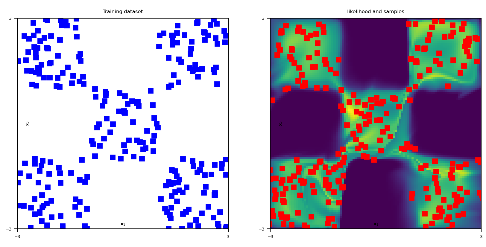
Figure 1. Results of a normalizing flow on a ‘chessboard’ dataset. On the left, the training dataset, and on the right the probability distribution estimated by the model and a few samples (red dots) generated by the model.
These approaches give pretty good results as we can see in Figure 1. Nevertheless their huge drawback is the condition forcing the latent space dimension to be equal to the dimension of the orignal probability distribution : this makes these approaches almost unusable in practice.
Variational autoencoders
Variational autoencoders algorithms also try to evaluate the log-likelihood of a generator. Nevertheless they accomplish that with a method that does not require anything on the latent space dimension q, which makes them much more useful in practice [5].
VAE algorithms rely on the Bayes-rule of conditional probabilities: the likelihood p_{\theta}(x) depends on the values p_{\mathcal{Z}}(z) and p_{\theta} (x|z) which are both easy to calculate and on the value p_{\mathcal{Z}} (z |x).
The function z \mapsto p_{\mathcal{Z}} (z |x), called the posterior distribution, is harder to evaluate: this is why we approach it with a second neural network. Starting from a point x, it gives us an approximation q_{\psi}( \_ | x) of the posterior distribution p_{\mathcal{Z}} ( \_ |x).
Replacing the posterior by its approximation in the Bayes conditional probabilities formula gives us a lower bound of the log-likelihood, that also measures the quality of the approximation q_{\psi}. Therefore we can use this quantity as a loss function for both neural networks.
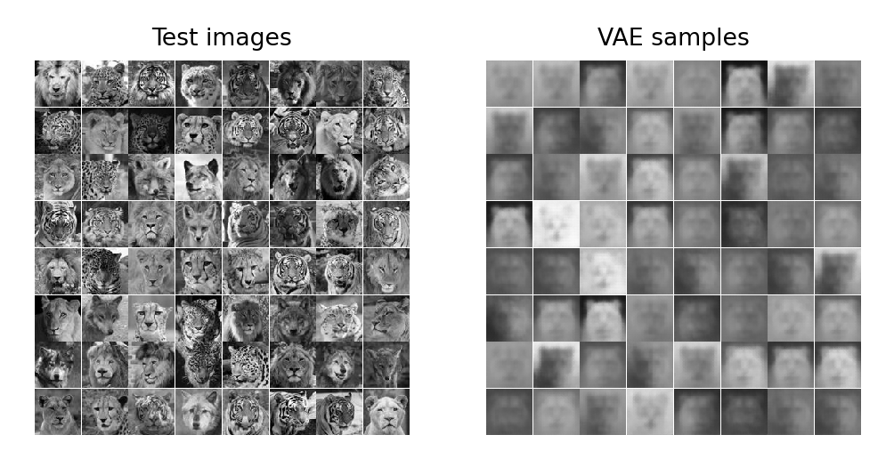
Figure 2. On the left, some pictures of animals which were in the training dataset. On the right, a few samples generated by the VAE algorithm.
This model is quite hard to train but we present some results in Figure 2. If we can recognize the shapes of the animals, the results are way too blurry to be realistic. We had to make approximations in the calculation of the posterior which caused an oversimplification of the problem. The model is then unable to learn how to represent the eyes or the dots of the animals, and how to fill their faces.
Generative Adversarial Networks
Finally, generative adversarial networks are the most promising algorithms. Instead of trying to maximize the log-likelihood, we will try to minimize the distance between the spaces of the probability distributions.
A first approach, presented by Ian Goodfellow in [8] consists in training simultaneously a generator g_{\theta} and a discriminator d_{\phi} mapping from the training variables space to [0,1]. This discriminator is supposed to be able to tell whether an image is a fake one created by the generator (in which case it would be close to 0) or a real one (making it close to 1). This algorithm wants to improve simultaneously the generator and the discriminator.
We can define the loss function :
J_{GAN}(\theta, \phi) = \mathbb{E}_{x \sim \mathcal{X}} \left( \log d_{\phi}(x) \right) + \mathbb{E}_{z \sim \mathcal{Z}} \left(\log (1 - d_{\phi}(g_{\theta} (z))) \right)The first term of the sum evaluates how good the discriminator is to identify real samples : the more real samples the discriminator identify as real, the higher it is. The second term evaluates how confused the discriminator is by the generator : the more fake samples it identifies as real, the lower this quantity is. Therefore we can use this function to train the generator neural network and the opposite of this function to train the discriminator neural network.
This model can be very efficient but is also tricky to train : the discriminator and the generator must improve at the same ‘speed’, or else one will soon outperform the other causing the algorithm to converge much slower, or even to fail. To avoid some of these problems, we can also change the loss function to another one defined in [9] based on the Wasserstein distance between the two probability distributions. One of its advantages is to prevent the generator to exploit a local weakness of the discriminator.
GANs are by far the most performing generative models and have proven their usefulness in numerous situations. We can think for instance of deepfakes. Generative models are able to create very realistic human pictures from scratch, which can have a lot of applications : creating a mass of fake social media profiles, replacing somebody’s face by another in a video…
They are also able to create photos even more detailed than the original ones : it is known as super resolution. Some of the models presented in [13] are able to create realistic pictures with a better resolution than the ones of the training dataset. This can be used for scientific applications, for instance in the case of astrophysics presented in [12], where GANs are used to recover features from noisy galaxy photos.
It can also be used to ‘create art’, ie to change the style of a picture : the article [11] presents a model capable of turning a picture of a city in a painting of Picasso, Van Gogh or Munch for instance ; see Figure 3.
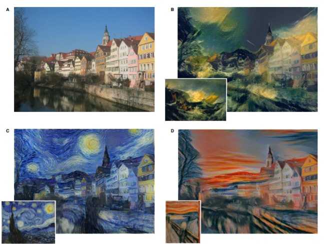
Figure 3. Pictures extracted from [11]; A is a photo depicting the Neckarfront in Tubingen, Germany, B, C and D are the photographs obtained with the styles of The Shipwreck of the Minotaur by J.M.W. Turner , The Starry Night by Vincent van Gogh and The Scream by Edvard Munch respectively.
For all these reasons, generative modelling algorithms are a widely studied subject nowadays. There is no doubt these models will keep getting better and better and find even more applications in the future.
References
[1] Lars Ruthotto, Eldad Haber, An Introduction to Deep Generative Modeling (2021), CoRR, Vol. abs/2103.05180, https://arxiv.org/abs/2103.05180 [2] Tian Qi Chen, Yulia Rubanova, Jesse Bettencourt, David Duvenaud. Neural Ordinary Differential Equations (2019), CoRR, Vol. abs/1806.07366, http://arxiv.org/abs/1806.07366 [3] George Papamakarios, Eric Nalisnick, Danilo Jimenez Rezende, Shakir Mohamed, Balaji Lakshminarayanan, Normalizing Flows for Probabilistic Modeling and Inference, (2021) Journal of Machine Learning Research, Vol. 22, No. 57, pp. 1-64, http://jmlr.org/papers/v22/19-1028.html [4] Derek Onken, Samy Wu Fung, Xingjian Li, Lars Ruthotto, OT-Flow: Fast and Accurate Continuous Normalizing Flows via Optimal, Transport (2020), CoRR, Vol. abs/2006.00104, http://arxiv.org/abs/2006.00104 [5] Diederik P. Kingma, Max Welling, An Introduction to Variational Autoencoders (2019), CoRR, Vol. abs/1906.02691, http://arxiv.org/abs/1906.02691 [6] Anand Sharma, Vedant Rastogi, Spam Filtering using K mean Clustering with Local Feature Selection Classifier (2014), International Journal of Computer Applications,Vol. 108, pp. 35-39 [7] Seyedmehdi Hosseinimotlagh and Evangelos E. Papalexakis, Unsupervised Content-Based Identification of Fake News Articles with Tensor Decomposition Ensembles” (2018), http://snap.stanford.edu/mis2/files/MIS2_paper_2.pdf [8] Ian J. Goodfellow, Jean Pouget-Abadie, Mehdi Mirza, Bing Xu, David Warde-Farley, Sherjil Ozair, Aaron Courville, Yoshua Bengio, Generative Adversarial Networks (2014), eprint=1406.2661 [9] Martin Arjovsky, Soumith Chintala, Léon Bottou, Wasserstein GAN (2017) eprint=1701.07875, [10] Gábor J. Székely, Maria L. Rizzo, Testing for equal distributions in high dimensions, InterStat (2004) [11] Gatys, Leon A., Ecker, Alexander S., Bethge, Matthias, Image Style Transfer Using Convolutional Neural Networks (2016) Proceedings of the IEEE Conference on Computer Vision and Pattern Recognition (CVPR)}, [12] Schawinski, Kevin, Zhang, Ce, Zhang, Hantian, Fowler, Lucas, Santhanam, Gokula Krishnan. Generative Adversarial Networks recover features in astrophysical images of galaxies beyond the deconvolution limit (2017). Monthly Notices of the Royal Astronomical Society: Letters, pp. slx008, ISSN=1745-3933, url=http://dx.doi.org/10.1093/mnrasl/slx008, DOI: 10.1093/mnrasl/slx008 [13] Christian Ledig, Lucas Theis, Ferenc Huszar, Jose Caballero, Andrew Cunningham, Alejandro Acosta, Andrew Aitken, Alykhan Tejani, Johannes Totz, Zehan Wang, Wenzhe Shi. Photo-Realistic Single Image Super-Resolution Using a Generative Adversarial Network (2017), eprint=1609.04802 [14] Silhouette (clustering), http://en.wikipedia.org/wiki/Silhouette_(clustering)
![]()
More about: ERC DyCon project
|| See more posts at DyCon blog