Introduction to spherical geometry: postulates and Pythagoras’ theorem

Spain. 29.03.2022
Author: Elisa Affili

Introduction

In this post, we present some basic facts about the study of geometry on spheres. In fact, geometry on the sphere is surprisingly different from the one on the plane: for example, Pythagoras’ Theorem does not hold anymore! Here, we will present a version of Pythagoras’ Theorem for the sphere and we will show what links it has with the original one.

The misleading fifth postulate

Geometry is traditionally the branch of Mathematics that studies shapes and spatial relationships of bodies.
Its development originate from some real-world problems about the measurements of fields and territories. In the Ancient Greece, these questions gave rise to a rational, abstract discipline where statements were originated in a deductive way, with the exemption of few axioms, considered too fundamental to need proves. The main legacy of the knowledge developed in Ancient Greece on these topics are the 13 books of the Elements by Euclid.

The first book starts by enouncing the basic elements of geometry and the celebrated five postulates.
The basic elements are: the point, with is considered the element with no dimension; the segment of line, which is the object with only one dimension; and the plane, which has two dimensions.
Looking at these three objects, we already see that the Ancient Greeks restricted their studies to flat figures, ignoring different type of surfaces.

Then, the book goes on with the statement of the postulates, including the famous Euclid’s fifth postulate, which original statement is:

Postulate (Euclid’s fifth postulate). If a straight line falling on two straight lines makes the interior angles on the same side of it taken together less than two right angles, then the two straight lines, if produced indefinitely, meet on that side on which the sum of angles is less than two right angles.

This is also called the Parallels’ postulate, since it’s equivalent to the following formulation by Playfair (1748 – 1819):

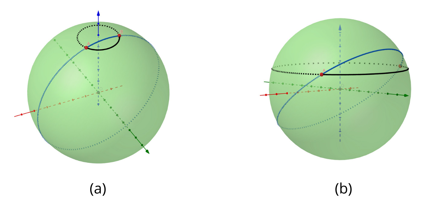
Figure 1. Arcs of minimal length connecting two points (in blue) versus other arcs of circumferences on the sphere

Postulate. In a plane, given a line and a point not belonging to it, at most one line parallel to the given line can be drawn through the point.

Euclid’s fifth postulate has always raised doubts about its nature. In fact, in the books of the Elements, this postulate is first used in Proposition 28. Hence, many mathematician sensed that it was not really fundamental. Prominent scientists, including the astronomer Ptolemy and the inventor of the trigonometry, Nasir al-Din al-Tusi, tried to prove Euclid’s postulate through other postulates, but eventually failed. It was only in the XIX century that the issue was understood: by rejecting the fifth postulate, it was possible to create other axiomatic geometries, based on surfaces other than the plane.

Postulates on the sphere

When thinking about geometry on the sphere, we work with different basic elements. One basic element is obviously the sphere. Another basic element is again the point, but we have to stress that each point comes an \emph{antipodal}, that will relate differently than the rest of the points. In particular, we state that the surface of the sphere is the union of antipodal couples of points, such that each point is part of one and only one couple and the elements of each couple are distinct.

For the third basic element, we cannot use straight lines any more, since they don’t lie on the surface of the sphere. Among all possible paths between two points, we want to choose the one of minimal length. This correspond to an arc of a maximal circle on the sphere. To convince ourself of this, we have a look at Figure 1. In blue, there is a circle which has the same radius as the sphere and in black, a circle with a strictly smaller radius passing through the points $A$ and $B$. The difference in the length of the path is evident when one consider very small radius for the black circle (as in (a)), but is present in all cases. In fact, maximal circles just follow the “natural” curvature of the surface, while smaller circles have some extra curvature and therefore they are not minimal.

Then, the postulate on which spherical geometry is based are:
1. Through each couple of points which are not antipodals there exits one and only one maximal circle.
2. Each arc of a maximal circle can be prolonged indefinitely at both extrema.
3. A circle can be drawn with any centre and any radius.
4. All right angles are equal to one another.
5. Any couple of distinct maximal circles meets in two antipodal points.

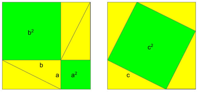
Figure 2. Visual proof of Pythagoras’ theorem

Of course, being the surface finite, we have some great difference with respect to what we are used on the plane, and some of these postulate may seem counter-intuitive. For example, some people find the second postulate hard to believe, since each circle has a finite length. However, what the second postulate states is that a circle has no extrema, that means, it is not bounded and has no border, even if it has a finite length. In a similar way, in the third postulate, we may choose a radius of any length, and then “roll” around the sphere if it’s longer than a maximum circle. This also means that, given a circle on the sphere, we can attribute to it two distinct centres and infinitely many radia.

We are also able to define angles on the sphere. To do that, we start from two maximal circles on the sphere and we have that:

Definition 1
An angle or spherical lune is the part of the sphere bounded by two half maximal circles with common extrema.
The angles may be measured in radiant.

To define a triangle on the sphere, we pass by a construction; first, we define

Definition 2
Given three non complanar half-lines staring from a common origin, a thriedron is the convex part of space bounded by the three planes originated by three half lines taken two by two.

Then,

Definition 3
A spherical triangle is the intersection of the sphere and a thriedron with origin in the centre of the sphere.

Notice that the side of a spherical triangle are arc of maximal circumferences on the sphere, since they are the intersections between the sphere and a plane passing through the centre of the sphere.
It has to be so: in fact, the sides of a triangle must be “straight lines” for the sphere, which are arcs of maximal circles.

The lack of parallel lines ruins the arguments in the proof of many basic theorems, including Pythagoras’ one:

Theorem(Pythagoras’ Theorem)
Given a planar triangle $\triangle ABC$ with length of the sides $a$, $b$ and $c$, which has a right angle opposite to the side $c$, we have

$c^2= a^2+b^2.$

There are many proof of this result, for example the visual one that you can find in Figure 2, that clearly makes use of the existence of parallels.

Also, it is easy to find a counterexample to Pythagoras’ Theorem on the sphere:

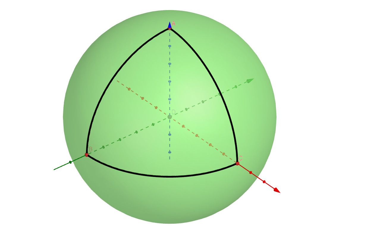
Figure 3. Counterexample to planar Pythagoras’ Theorem

Counterexample. Let us consider the spherical triangle given by an eighth of the surface of the sphere. More precisely, given three maximal circumferences of the sphere that are two by two perpendicular, consider a spherical triangle $\triangle ABC$ with sides of length one quarter of the maximal circumference, as in Figure 3. Then, $\triangle ABC$ is a right-angled triangle (it even has three right angles!), but the lengths of its sides do not satisfy Pythagoras’ Theorem.

3. Pythagoras’ Theorem on the sphere

We now state Pythagoras’ Theorem for spherical triangles:

Theorem 1.
On the sphere of centre $O$ and radius $R$, let $\triangle ABC$ be a spherical triangle with $\widehat{ACB}$ a right angle with opposite side of length $c$, and the other two sides of length $a$ and $b$. Then, we have

$\cos\left(\frac{c}{R}\right)=\cos\left(\frac{a}{R}\right) \cos \left(\frac{b}{R}\right).$

We notice that the given formula is still a relation between the length of the side of the triangle, more precisely between the hypotenuse and the other two sides. Further justification on the reason why this corresponds to Pythagoras’ Theorem on the plane will be given in the next section. Now, we will give the proof of the theorem.

Euclidian coordinates given some angles
Before giving the proof of Pythagoras’ Theorem for spherical triangle, we recall that we can give the euclidian coordinate of a point on a sphere if we know what angles it forms with the $xy-$ and $xz-$planes (which are also called spherical coordinates of the point).

On the sphere of centre $O$ and radius $R$, let us take $A$ a point and $P$ its projection on the $xy-$plane. Let us call $B$ the point

$B = \left( \begin{array}{l} R \\ 0 \\ 0 \end{array} \right),$

and let $\widehat{BOP}=\psi$ and $\widehat{POA}=\phi$. Then, looking at the plane containing $O$, $A$ and $P$ (see Figure 4), we see that the $z-$coordinate of $A$ is $z_A=R \sin \phi$ and we have that $P$ lies on the circle of centre $O$ and radius $R\cos \phi$.

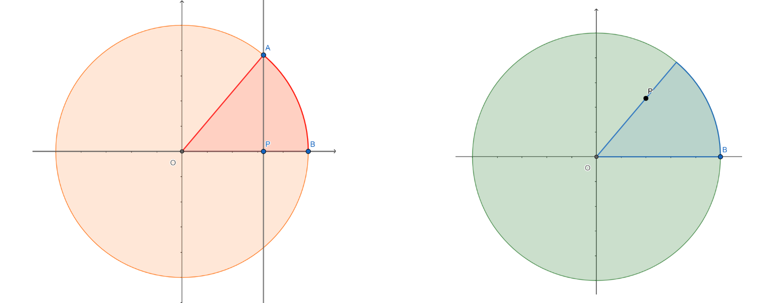
Figure 4. Projections on the plane containing $P$ and $A$ and on the $xy-$plane. In red, the angle $\phi$ and in blue, the angle $\psi$.

 

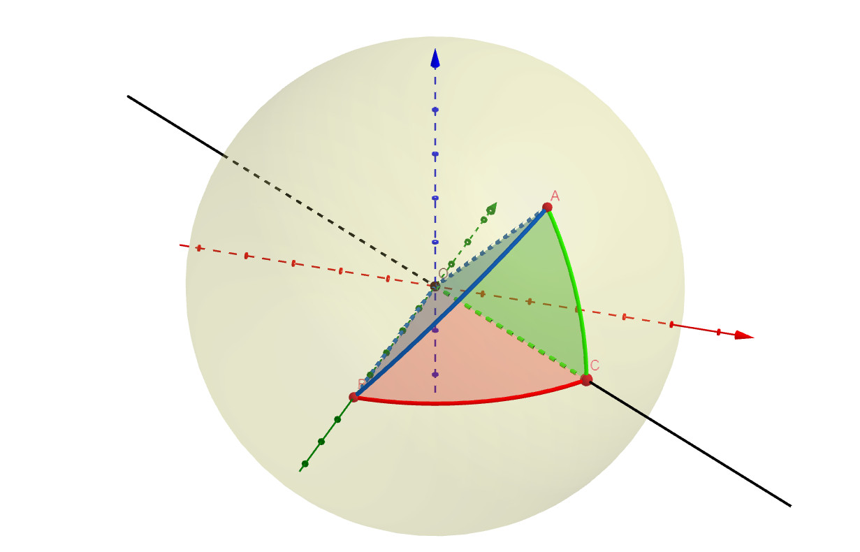
Figure 5. A triangle with a right angle in $C$.

Then, looking at the $xy-$plane containing $O$, $B$ and $P$, we see that the coordinates of $P$ are

$P = \left( \begin{array}{l} R\cos \phi \cos \psi \\ R\cos \phi \sin \psi \\ 0 \end{array} \right).$

So, the coordinates of $A$ are

$A= \left( \begin{array}{l} R \cos \phi \cos \psi \\ R \cos \phi \sin \psi \\ R \sin \phi \end{array} \right).$

Proof of Pythagoras’ Theorem on the sphere
Let us call the angles
• $\widehat{AOB}=\theta$,
• $\widehat{AOC}=\phi$,
• $\widehat{COB}=\psi$.

First, let us notice that the measure in radiant of $\theta$ is

$\theta = \frac{c}{R}$

since the side $AB$ of length $c$ is an arc of maximal circumference of the sphere. Similarly,

$\phi = \frac{b}{R} \qquad \text{and} \qquad \psi = \frac{a}{R}.$

Then, the claim becomes

$\cos\theta=\cos\phi \cos \psi.$

 

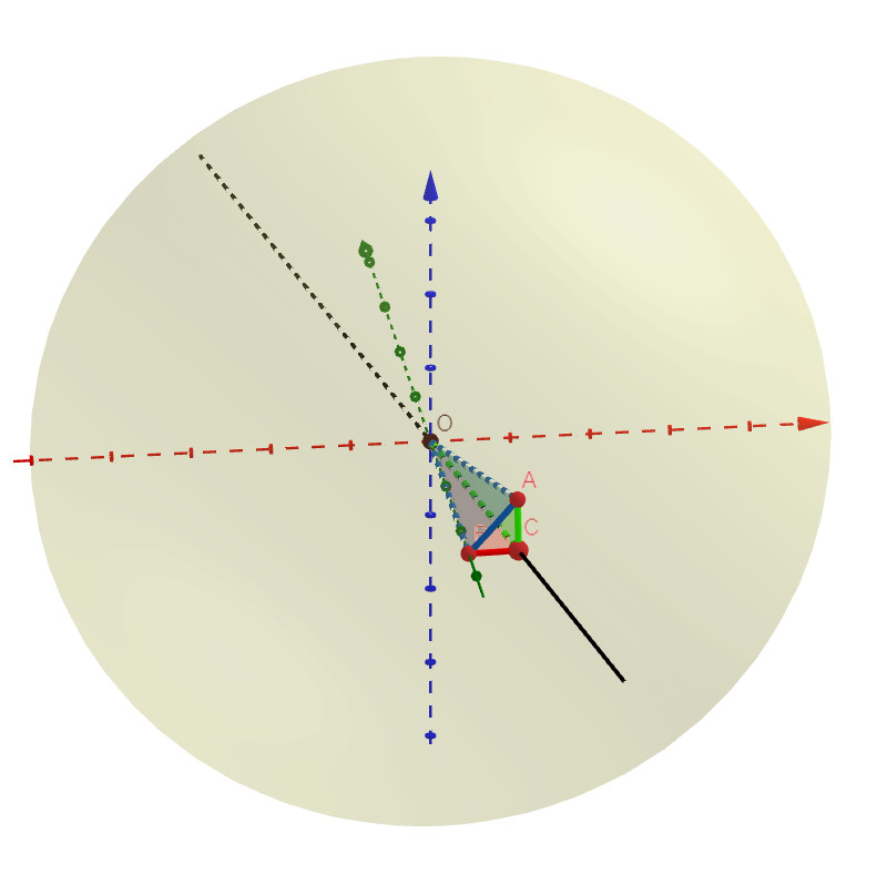
Figure 6. A right triangle of small area. With respect to the triangle in Figure 5, this triangle looks much more like a planar triangle.

Since the arc $AC$ is perpendicular to the $xy-$plane, the coordinates of the point $A$ are:

$A= \left( \begin{array}{l} R \cos \phi \cos \psi \\ R \cos \phi \sin \psi \\ R \sin \phi \end{array} \right).$

Now let us write the vectorial product $\overset{\longrightarrow}{OA}\cdot \overset{\longrightarrow}{OB}$ in two different ways.

First, by using the euclidian coordinates, we get

$\overset{\longrightarrow}{OA}\cdot \overset{\longrightarrow}{OB}= R^2 \cos \psi \cos \phi .$

Then, recalling that the product of two vectors is the product of the norms by the cosine of the angle between the vectors, we get

$\overset{\longrightarrow}{OA}\cdot \overset{\longrightarrow}{OB}= R^2 \cos \theta.$

Putting together the last two, we get the formula we wished for.

4. Recovering Pythagoras’ theorem on the plane

On a sphere of radius $R$, let us take a little spheric cap of area, let’s say, 1. Then, let us increase $R$ while keeping the area of the cap fixed: the cap will look smaller and smaller when compared to the surface of the entire sphere. Also, it will appear “flatter” compared to the caps of smaller spheres.
So, it means that a spherical triangle $\triangle ABC$ on this cap will also be quite flat and its angles and sides will be small.

So, if our Theorem 1 corresponds to Pythagoras’ Theorem, then for a “quite flat” triangles the relation

$\cos\left(\frac{c}{R}\right)=\cos\left(\frac{a}{R}\right) \cos \left(\frac{b}{R}\right)$

must be close to $c^2=a^2+b^2$.

As we said before, the quantities $\frac{a}{R}$, $\frac{b}{R}$ and $\frac{c}{R}$ get smaller and approach 0 as $R$ gets bigger. Now, we look at the function $\cos x$ as $x$ tends to 0. Thanks to some classical estimates, called Taylor series, we can write the approximation

$\cos x \approx 1- \frac{x^2}{2}$

which is true for small values of $x$. Now, let us write the formula of spherical Pythagoras’ Theorem with this approximation, obtaining

$1 -\frac{1}{2} \left(\frac{c}{R}\right)^2 \approx \left[ 1 -\frac{1}{2} \left(\frac{a}{R}\right)^2 \right] \left[ 1 -\frac{1}{2} \left(\frac{b}{R}\right)^2\right].$

Let us now develop the calculations. We get that

${1} -\frac{1}{2} \left(\frac{c}{R}\right)^2 \approx {1} -\frac{1}{2} \left(\frac{a}{R}\right)^2 -\frac{1}{2} \left(\frac{b}{R}\right)^2 +{ \frac{1}{4} \left(\frac{ab}{R^2}\right)^2}.$

We cancel out the $1$ and we multiply everything by $-\frac{1}{2}$, getting

$\left(\frac{c}{R}\right)^2 \approx \left(\frac{a}{R}\right)^2 + \left(\frac{b}{R}\right)^2 -\frac{1}{2}\left(\frac{ab}{R^2}\right)^2.$

Now we multiply everything by $R^2$ and get

$c^2 \approx a^2 + b^2 -\frac{1}{2}\left(\frac{a^2b^2}{R^2}\right).$

We are very close to classical Pythagoras’ formula! Our last observation is that, when $R$ gets larger and larger, the quantity $\frac{a^2b^2}{R^2}$ approaches 0. Then we have that

$c^2 \approx a^2 + b^2,$

as wished.