Spain 12.08.2022
Optimal control of mixed local-nonlocal elliptic PDE with singular boundary-exterior data
Author: Jean-Daniel Djida
In this post we are interested in optimal control problem of the mixed local-nonlocal elliptic problem. We prove well-posedness and regularity results of the associated elliptic with singular boundary-exterior data.
Secondly, we show the existence of optimal solutions of associated optimal control problem, and we characterize the optimality conditions.
1 Mixed local-nonlocal problem
Let \Omega\subset\mathbb{R}^{N} (N\ge 1) be a bounded domain with a smooth boundary \partial \Omega. We consider the following initial-boundary-exterior value problem:
\begin{cases} \mathscr{L}\psi = 0 & { in }\; \Omega,\\ \psi=u_1& { on }\;\partial \Omega,\\ \psi = u_2 & { in }\; (\mathbb{R}^{N}\setminus \Omega), \\ \end{cases} (1.1)
Here, the operator \mathscr{L} is given by
\mathscr{L} \coloneqq - \Delta + (-\Delta)^{s},\qquad 0 \lt s \lt 1, (1.2)
In (1.2), \Delta is the classical Laplacian and (-\Delta)^s (0 \lt s \lt 1) denotes the fractional Laplace operator given formally by the following singular integral:
(-\Delta)^s\psi= {P.V.}\;C_{N,s}\int_{\mathbb{R}^{N}}\frac{\psi(x)-\psi(y)}{|x-y|^{N+2s}}\;dy,
where C_{N,s} is a normalization constant depending only on N and s and given by
C_{N,s}\coloneqq \frac{s2^{2s}\Gamma\left(\frac{2s+N}{2}\right)}{\pi^{\frac{N}{2}}\Gamma(1-s)}.
Integro-differential equations of the form (1.1) arise naturally in the study of stochastic processes with jumps. The generator of an N-dimensional Lévy process has the following general structure:
\mathscr{L} u = \alpha \sum_{i, j} a_{i j} \partial_{i j} u+\gamma \sum_{j} b_{j} \partial_{j} u+ \beta \int_{\mathbb{R}^{N}}(u(x+\xi)-u(x)- \xi \cdot \nabla u(x)) \chi_{B_{1}}(\xi) \mathrm{d} \nu(\xi), (1.3)
where \nu is the Lévy measure and satisfies \int_{\mathbb{R}^{N}} \min \left\{1,|\xi|^{2}\right\} \mathrm{d} \nu(\xi) \lt +\infty, and \chi_{B_{1}} is the usual characteristic function of the unit ball B_{1} of \mathbb{R}^{N}. The first term of (1.3) on the right-hand side corresponds to the diffusion, the second one to the drift, and the third one to the jump part.
For the above reasons, the study of the operator \mathscr{L} with diffusion, drift and jump components appears quite intriguing. Here, we focus on the case \mathscr{L} \coloneqq - \alpha \Delta + (-\Delta)^{s}, obtained from (1.3) by setting a_{i j}=\alpha^{-1} \delta_{i j}, \gamma = 0 and \nu given by the symmetric kernel \beta^{-1}|x-\xi |^{-N-2s}.
Indeed, the particular case when \nu=0, namely when there are no jumps, \mathscr{L} turns into a classical second-order differential operator. Foremost, for \gamma = 0, the operator \mathscr{L} reduced to the Laplace operator obtained from the brownian motion (see Figure 1). Here, \psi(x)=\mathbb{E}\left(u_{1}\left(B_{\tau}^{x_{0}}\right)\right)=\mathbb{E}(\text { pay off }) solves:
\begin{cases} -\Delta \psi = 0 & { in }\; \Omega,\\ \psi=u_1 & { on }\;\partial \Omega, \end{cases}
On the other hand, the case when the process has no diffusion and no drift has attracted a lot of attention recently. In particular, one of the most prominent operators belonging to this class is the fractional Laplacian (-\Delta)^{s}, which turns out to be the infinitesimal generator of isotropic s-stable Lévy processes. Here, \psi(x) =\mathbb{E}\left(u_{2}\left(X_{\tau}^{\chi_{0}}\right)\right)=\mathbb{E}(\text { pay off }) solves:
\begin{cases} (-\Delta)^{s}\psi = 0 & { in }\; \Omega,\\ \psi = u_2 & { in }\; (\mathbb{R}^{N}\setminus \Omega), \\ \end{cases}
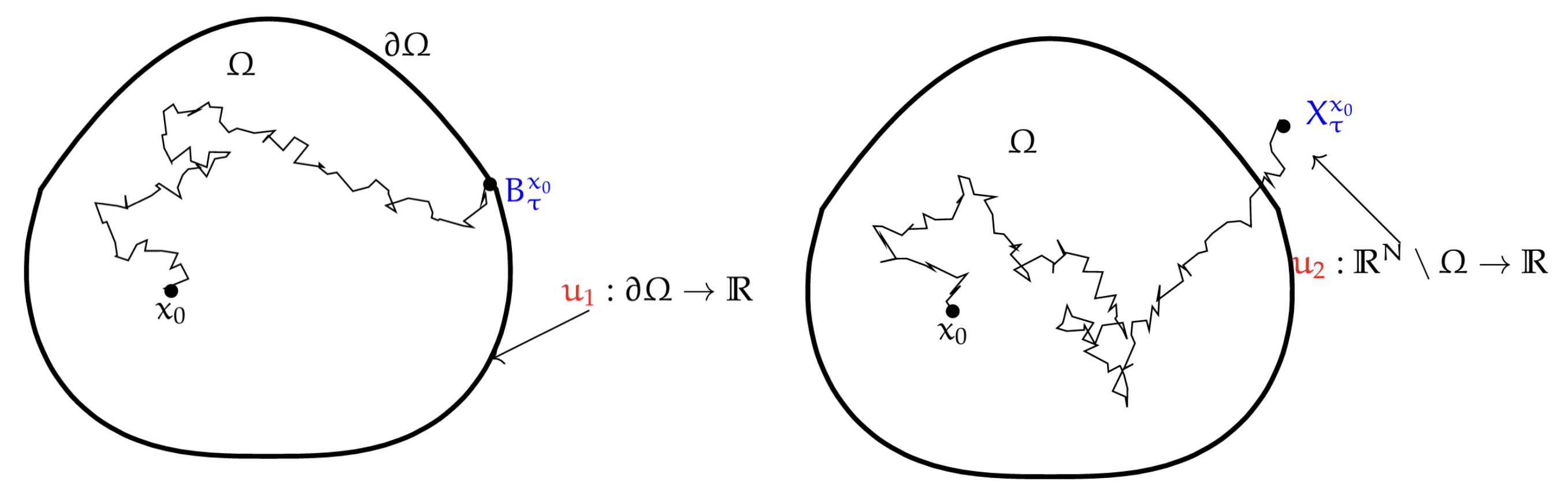
Figure 1. On the left, brownian motion leading by local operator and on the right we have Lévy process leading to nonlocal operator.
Goal:
For non-smooth boundary-exterior data, we shall introduce the notion of solutions by transposition (or very-weak solutions) of (1.1), study their existence and regularity. Next, in this direction reads that if u_1\in L^2(\partial \Omega), u_2\in L^2(\mathbb{R}^{N}\setminus \Omega) and 0 \lt s\le 3/4, then the associated very-weak solution \psi of (1.1) belongs to H^{1/2}(\Omega)\cap L^2(\mathbb{R}^{N}). Finally, study the existence of optimal solutions to optimal control problems involving the mixed operator \mathscr{L} with singular Dirichlet boundary-exterior data, and to characterize the associated optimality conditions. More precisely, we shall consider the following two different optimal control problems:
\min_{(u_1,u_2)\in \mathcal{Z}_{ad}} \mathcal{J}((u_1,u_2)), (1.4)
subject to the constraint that the state \psi\coloneqq \psi(u_1,u_2) solves the parabolic system (1.1). We recall that the control (u_1,u_2) \in \mathcal{Z}_{ad} with \mathcal{Z}_{ad} being a closed and convex subset of Z_{D}\coloneqq L^2(\partial \Omega) \times L^{2}(\mathbb{R} \ \Omega), which is endowed with the norm given by
\|(u_{1},u_{2})\|_{ Z_{D}}=\left(\|u_{1}\|^2_{L^2(\partial \Omega)}+\|u_{2}\|^2_{ L^{2}(\mathbb{R}^{N}\setminus \Omega)}\right)^{\frac 12}.
The functional \mathcal{J} is given by
\mathcal{J}(u_1,u_2)\coloneqq \frac{1}{2}\|\psi((u_{1},u_{2}))-z_d^1\|_{L^2(Q)}^2 + \frac{\beta}{2}\|(u_{1},u_{2})\|^{2}_{\mathcal{Z} _{D}} (1.5)
where \beta>0 is a real number, z_d^1\in L^2(Q) , z_d^2\in H^{-1}(\Omega),
and
\|\phi\|^2_{H^{-1}(\Omega)}:=\langle (-\Delta_D)^{-1}\phi,\phi\rangle_{H^1_0(\Omega),H^{-1}(\Omega)}.
Here, -\Delta_D is the realization in L^2(\Omega) of the Laplace operator -\Delta with the zero Dirichlet boundary condition.
2 Notations and Preliminaries
Let \Omega\subset\mathbb{R}^{N} be an arbitrary open set. Given 0 \lt s \lt 1 a real number, we let
H^{s}(\Omega)\coloneqq \left\{w \in L^2(\Omega):\;\int_{\Omega}\int_{\Omega}\frac{|w(x)-w(y)|^2}{|x-y|^{N+2s}}\;\mathrm{d}x\mathrm{d}y\lt \infty\right\},
and we endow it with the norm defined by
\|w\|_{H^{s}(\Omega)}\coloneqq\left(\int_{\Omega}|w(x)|^2\;\mathrm{d}x+ \int_{\Omega}\int_{\Omega}\frac{|w(x)-w(y)|^2}{|x-y|^{N+2s}}\;\mathrm{d}x\mathrm{d}y\right)^{\frac 12}.
We set
H_0^{s}(\Omega)\coloneqq\Big\{w\in H^{s}(\mathbb{R}^{N}):\;w=0\; { in }\;\mathbb{R}^{N}\setminus\Omega\Big\}.
Then, H_0^{s}(\Omega) endowed with the norm
\|w\|_{H_0^{s}(\Omega)}=\left(\int_{\mathbb{R}^{N}}\int_{\mathbb{R}^{N}} \frac{|w(x)-w(y)|^2}{|x-y|^{N+2s}}\;\mathrm{d}x\, \mathrm{d}y\right)^{1/2}, (2.1)
is a Hilbert space. We let H^{-s}(\Omega)\coloneqq (H_0^s(\Omega))^\star be the dual space of H_0^s(\Omega) with respect to the pivot space L^2(\Omega), so that we have the following continuous and dense embeddings:
H_0^{s}(\Omega) continuous embedded in L^2(\Omega) continuous embedded in H^{-s}(\Omega). (2.2)
Next, for \varphi\in H^{s}(\mathbb{R}^{N}) we introduce the {\em nonlocal normal derivative \mathcal N_s} given by
\mathcal N_{s}\varphi(x)\coloneqq C_{N,s}\int_{\Omega}\frac{\varphi(x)-\varphi(y)}{|x-y|^{N+2s}}\; \mathrm{d}y,~~~~x\in\mathbb{R}^{N}\setminus\overline{\Omega}. (2.3)
It is worthwhile noticing that the operator \mathcal N_s maps H^s(\mathbb{R}^{N}) into H_{\rm loc}^s(\mathbb{R}^N\setminus\overline{\Omega}).
Furthermore, if u\in H_0^1(\Omega) and (-\Delta)^s u\in L^2(\Omega), then \mathcal N_su\in L^2(\mathbb{R}^N\setminus\overline{\Omega}), and there is a constant C>0 such that
\|\mathcal N_su\|_{L^2(\mathbb{R}^N\setminus\overline{\Omega})}\le C\|u\|_{H_0^1(\Omega)}. (2.4)
To introduce the notion of solution of our problem (1.1), we need the following integration by parts formula.
Let \varphi\in H^{s}(\mathbb{R}^{N}) be such that (-\Delta)^s \varphi\in L^2(\Omega) and \mathcal N_s\varphi\in L^2(\mathbb{R}^N\setminus\overline{\Omega}). Then, for every \psi\in H^{s}(\mathbb{R}^{N}), the identity
\frac{C_{N,s}}{2}\int\int_{\mathbb{R}^{2N}\setminus(\mathbb{R}^{N}\setminus \Omega)^2} \frac{(\varphi(x)-\varphi(y))(\psi(x)-\psi(y))}{|x-y|^{N+2s}}\;\mathrm{d}x\, \mathrm{d}y =\int_{\Omega}\psi(-\Delta)^s\varphi\;\mathrm{d}x+\int_{\mathbb{R}^{N}\setminus \Omega}\psi\mathcal N_s \varphi\;\mathrm{d}x
holds. Observing that
\mathbb{R}^{2N}\setminus(\mathbb{R}^{N}\setminus\Omega)^2=(\Omega\times\Omega)\cup (\Omega\times(\mathbb{R}^{N}\setminus\Omega))\cup((\mathbb{R}^{N}\setminus\Omega)\times\Omega),
we have that if \varphi=0 in \mathbb{R}^{N}\setminus \Omega or \psi=0 in \mathbb{R}^{N}\setminus \Omega, then
\int\int_{\mathbb{R}^{2N}\setminus(\mathbb{R}^{N}\setminus\Omega)^2} \frac{(\varphi(x)-\varphi(y))(\psi(x)-\psi(y))}{|x-y|^{N+2s}}\mathrm{d}x\,\mathrm{d}y =\int_{\mathbb{R}^{N}}\int_{\mathbb{R}^{N}}\frac{(\varphi(x)-\varphi(y))(\psi(x)-\psi(y))}{|x-y|^{N+2s}}\mathrm{d}x\,\mathrm{d}y.
Throughout the remainder of the note, we shall let the bilinear form \mathcal F:H_0^{s}(\Omega)\times H_0^{s}(\Omega)\to\mathbb{R} be given by
\mathcal{F}(\varphi,\psi)\coloneqq \frac{C_{N,s}}{2} \int_{\mathbb{R}^{N}}\int_{\mathbb{R}^{N}}\frac{(\varphi(x)-\varphi(y))(\psi(x)-\psi(y))}{|x-y|^{N+2s}}\;\mathrm{d}x\, \mathrm{d}y. (2.5)
Next, we introduce the classical first order Sobolev space
H^1(\Omega):=\left\{u\in L^2(\Omega):\;\int_{\Omega}|\nabla u|^2\;\mathrm{d}x \lt \infty\right\}
which is endowed with the norm defined by
\|u\|_{H^1(\Omega)}=\left(\int_{\Omega}|u|^2\;\mathrm{d}x+\int_{\Omega}|\nabla u|^2\;\mathrm{d}x\right)^{\frac 12}.
In order to study the solvability of (1.1), we shall also need the following function space
H_0^1(\Omega) \coloneqq \Big\{w \in H^1(\mathbb{R}^{N}) : w \equiv 0 in \mathbb{R}^{N}\setminus \Omega \Big\}, (2.6)
which is a (real) Hilbert space endowed with the scalar product
\int_{\Omega} \nabla w\cdot\nabla \varphi\,\mathrm{d}x,
and associated norm
\|\varphi\|_{H_0^1(\Omega)}\coloneqq \|\nabla \varphi\|_{L^2(\Omega)}. (2.7)
Furthermore, the classical Poincar\'{e} inequality holds in H_0^1(\Omega). That is, there is a constant C > 0 such that
\|\varphi\|_{L^2(\Omega)} \leq C\,\|\varphi\|_{H_0^1(\Omega)}\qquad \text{for all} \varphi\in H_0^1(\Omega). (2.8)
We shall denote by H^{-1}(\Omega) the dual space of H_0^1(\Omega) with respect to the pivot space L^2(\Omega) so that we have the following continuous and dense embeddings:
H_0^{1}(\Omega) continuous embedded in L^2(\Omega) continuous embedded in H^{-1}(\Omega).
Here also, if \Omega is bounded and has a Lipschitz continuous boundary, then by [4, Chapter 1]
H_0^1(\Omega)=\overline{\mathcal D(\Omega)}^{H^1(\Omega)}.
In addition, under the same assumption on \Omega, every function u\in H^1(\Omega) has a trace u|_{\partial \Omega} that belongs to H^{1/2}(\partial \Omega), and the mapping trace
H^1(\Omega)\to H^{\frac 12}(\partial \Omega),\;\; u\mapsto u|_{\partial \Omega} (2.9)
is continuous and surjective.
Throughout the remainder of the paper, without any mention, we shall assume that \Omega\subset\mathbb{R}^{N} is a bounded domain with a smooth boundary \partial \Omega. Under this assumption, we have the following continuous and dense embedding for every 0 \lt s \lt 1 (see e.g. [4]):
H_0^1(\Omega) continuous embedded in H_0^s(\Omega). (2.10)
In view of (2.7) and (2.10), we can deduce that
(\varphi,\psi)_{H_0^1(\Omega)}:=\mathcal{F}(\varphi,\psi)+ \int_\Omega \nabla \varphi\cdot\nabla \psi \, \mathrm{d}x (2.11)
defines a scalar product on H_0^1(\Omega) with associated norm
\|\varphi\|_{H_0^1(\Omega)}\coloneqq \left(\mathcal{F}(\varphi,\varphi)+ \int_\Omega |\nabla \varphi|^2\, \mathrm{d}x\right)^{\frac 12}. (2.12)
The norm given in (2.12) is equivalent to the one given in (2.7).
3 Well-posedness
In the part of this post we are interested in establishing some existence, uniqueness and regularity results of the state equation (1.1)
that will be needed in the proof of the existence of minimizers to the optimal control problem (1.4). We start with the following non-homogeneous Dirichlet problem associated with the operator \mathscr{L}, as defined in (1.2). That is,
\begin{cases} -\Delta w + (-\Delta)^{s}w = f\;\;& { in }\;\Omega,\\ w=g_1& { on }\;\partial \Omega,\\ w=g_2& { in }\;\mathbb{R}^{N}\setminus \Omega. \end{cases} (3.1)
To introduce our notion of solutions to the system (3.1), we start with the simple case g_1=0 on \partial \Omega and g_2=0 in \mathbb{R}^{N}\setminus \Omega.
Definition 3.1.
Let f\in H^{-1}(\Omega), g_2=0 in \mathbb{R}^{N}\setminus \Omega and g_1=0 on \partial \Omega. A function w\in H_0^1(\Omega) is said to be a \emph{weak solution of} (3.1) if for every function \varphi\in H_0^1(\Omega), the identity
\int_{\Omega} \nabla w\cdot\nabla \varphi\,\mathrm{d}x +\mathcal F(w,\varphi) = \langle f,\varphi\rangle_{H^{-1}(\Omega), H_0^1(\Omega)} (3.2)
holds, where we recall that the bilinear form \mathcal F has been defined in (2.5).
The following existence result can be established by using the notion of solution by transposition already discussed in [1, Theorem 1.1].
Definition 3.2.
Let f\in H^{-1}(\Omega), g_1\in L^2(\partial \Omega), and g_2\in L^2(\mathbb{R}^{N}\setminus \Omega). A function w\in L^2(\mathbb{R}^{N}) is called a very-weak solution of (3.1), if the identity
\int_{\Omega}w \mathscr{L}\varphi\;\mathrm{d}x= \langle f,\varphi\rangle_{H^{-1}(\Omega), H_0^1(\Omega)} -\int_{\partial \Omega}g_1\partial_\nu\varphi\;\mathrm{d}\sigma-\int_{\mathbb{R}^N\setminus\overline{\Omega}}g_2\mathcal N_s\varphi\;\mathrm{d}x (3.3)
holds, for every
\varphi\in \mathbb V:=\Big\{\varphi\in H_0^1(\Omega):\; \mathscr{L}\varphi\in L^2(\Omega)\Big\}.
We notice that Definition 3.2 of very-weak solutions makes sense if every function \varphi\in\mathbb V satisfies \partial_\nu\varphi \in L^2(\partial \Omega), and \mathcal N_s\varphi\in L^2(\mathbb{R}^N\setminus\overline{\Omega}). We have the following existence theorem.
Theorem 3.3 ([1])
Let 0 \lt s\le 3/4. Then, for every f\in H^{-1}(\Omega), g_1\in L^2(\partial \Omega) and g_2\in L^2(\mathbb{R}^{N}\setminus \Omega), the system (3.1) has a unique very-weak solution w\in L^2(\mathbb{R}^{N}) in the sense of Definition 3.2, and there is a constant C>0 such that
\|w\|_{L^2(\mathbb{R}^{N})}\le C\left(\|f\|_{H^{-1}(\Omega)}+\|g_1\|_{L^2(\partial \Omega)}+\|g_2\|_{L^2(\mathbb{R}^{N}\setminus \Omega)}\right). (3.4)
In addition, if g_1 and g_2 are as in Definition 3.2, then the following assertions hold.
• Every weak solution of (3.1) is also a very-weak solution.
• Every very-weak solution of (3.1) that belongs to H^1(\mathbb{R}^{N}) is also a weak solution.
Remark 3.4.
We observe the following facts.
(a) We notice that in Definition 3.2 of very-weak solutions, we do not require that the function w has a well-defined trace on \partial\Omega and that w|_{\partial\Omega}=g_1, for that reason the regularity of w cannot be improved.
(b) But if w has a well-defined trace on \partial\Omega and w|_{\partial\Omega}=g_1\in L^2(\partial \Omega), then the regularity of w can be improved. Indeed, using well-known trace theorems (see e.g. [3]) we can deduce that w\in L^2(\mathbb{R}^{N})\cap H^{1/2}(\Omega).
(c) If 0 \lt s\le 3/4, then \mathbb V\subset H^2(\Omega)\cap H_0^1(\Omega). Indeed, let \varphi\in\mathbb V. If 0 \lt s \lt 1/2, it follows from the proof of Theorem 3.3 Step 1 that \varphi\in H^2(\Omega)\cap H_0^1(\Omega). If 1/2\le s\le 3/4, then the proof of Theorem 3.3 Step 1 shows again that \varphi\in H^{3-2s}\cap H_0^1(\Omega). Using \cite{G-JFA}, we get that, in fact (-\Delta)^s\varphi\in L^2(\Omega). This implies that \Delta\varphi\in L^2(\Omega). Thus, \varphi\in H^2(\Omega)\cap H_0^1(\Omega) by using elliptic regularity results for the Laplace operator.
(d) Consider the following Dirichlet problem: Find u\in H_0^1(\Omega) satisfying
\mathscr{L}u =f\; { in } \Omega.
Due to the presence of the fractional Laplace operator (-\Delta)^s, even if f is smooth, classical bootstrap argument cannot be used to improve the regularity of the solution u. This follows from the fact that even if f is smooth enough, if 1/2\le s \lt 1, then a function v\in H_0^s(\Omega) satisfying (-\Delta)^sv=f in \Omega only belongs to \cap_{\varepsilon>0}H^{2s-\varepsilon}(\Omega) and does not belong to H^{2s}(\Omega).
(e) In the case 3/4 \lt s \lt 1, if the function g_1 is smooth, says, g_1\in H^{2s-3/2}(\partial \Omega), then we may replace (3.3) in the definition of very-weak solutions by the expression:
\int_{\Omega}w \mathscr{L}\varphi\;\mathrm{d}x= \langle f,\varphi\rangle_{H^{-1}(\Omega), H_0^1(\Omega)} -\langle g_1,\partial_\nu\varphi\rangle_{H^{2s-3/2}(\partial \Omega),H^{3/2-2s}(\partial \Omega)}
-\int_{\mathbb{R}^N\setminus\overline{\Omega}}g_2\mathcal N_s\varphi\;\mathrm{d}x
holds, for every \varphi\in\mathbb V. In that case, Theorem 3.3 will be valid for every 0 \lt s \lt 1. But recall that the main objective of the paper is to study the minimization problem (1.4) and our control function u_1 does not enjoy such a regularity.
4 Optimal control problems of mixed local-nonlocal elliptic PDE
The aim of this section is to study the optimal control problem (1.4). Recall that
Z_{D} \coloneqq L^2(\partial \Omega)\times L^{2}(\mathbb{R}^{N}\setminus \Omega) is endowed with the norm given by
\|(u_{1},u_{2})\|_{ Z_{D}}=\Big(\|u_{1}\|^2_{L^2(\partial \Omega)}+\|u_{2}\|^2_{ L^{2}(\mathbb{R}^{N}\setminus \Omega)}\Big)^{\frac 12}. (4.1)
and U_{D}:=L^{2}(\Omega). We consider the following controlled equation:
\begin{cases} -\Delta \psi + (-\Delta)^{s}\psi = 0 & { in }\; \Omega,\\ \psi=u_1& { on }\;\partial \Omega,\\ \psi = u_2 & { in }\; \mathbb{R}^{N}\setminus \Omega , \end{cases} (4.2)
where the control (u_1,u_2) \in \mathcal{Z}_{ad} with \mathcal{Z}_{ad} being a closed and convex subset of Z_{D}.
In view of the above existence result given in Theorem 3.3, the following (solution-map) control-to-state map is well-defined
S: L^{2}(\partial \Omega) \times L^{2}(\mathbb{R}^{N}\setminus \Omega) \rightarrow L^{2}(\Omega), \quad\left(u_{1}, u_{2}\right) \quad \mapsto S\left(u_{1}, u_{2}\right)=\psi
and is linear and continuous. We also notice that for \left(u_{1}, u_{2}\right) \in Z_{D}:= L^{2}(\partial \Omega) \times L^{2}(\mathbb{R}^{N}\setminus \Omega), we have that \psi\coloneqq S\left(u_{1}, u_{2}\right) \in L^{2}\left(\mathbb{R}^{N}\right).
As a result we are interested in the following minimization problems:
\min _{\left(u_{1}, u_{2}\right) \in Z_{\mathrm{ad}}} \mathcal{J}\left(\left(u_{1}, u_{2}\right)\right):=\min_{\left(u_{1}, u_{2}\right) \in Z_{\mathrm{ad}}}\left(J\left(S\left(u_{1}, u_{2}\right)\right) +\frac{\beta}{2}\left\|\left(u_{1}, u_{2}\right)\right\|_{Z_{D}}^{2}\right) (4.3)
with
J\left(S\left(u_{1}, u_{2}\right)\right):=\frac{1}{2}\left\|\psi\left(\left(u_{1}, u_{2}\right)\right)-z_{\mathrm{d}}^{1}\right\|_{L^{2}(\Omega)}^{2} .
where \beta>0 is a real number, z_d^1\in L^2(\Omega) , z_d^2\in H^{-1}(\Omega), \psi:=\psi(u_1,u_2) is the unique very-weak solution of (4.2),
and
\|\phi\|^2_{H^{-1}(\Omega)}=\langle (-\Delta_D)^{-1}\phi,\phi\rangle_{H^1_0(\Omega),H^{-1}(\Omega)}.
Here, (-\Delta_D)^{-1}\phi=\varrho with \varrho the unique solution of the Dirichlet problem
-\Delta \varrho=\phi\; { in }\; \Omega\; { and }\; \varrho = 0\; { on }\; \partial \Omega.
4.1 The optimal control problem
In this section we consider the minimization problem (4.3) with the functional \mathcal{J}. We have the following existence result of optimal solutions.
Proposition 4.1
Let 0 \lt s\le 3/4, u_1\in L^2(\partial \Omega), and u_2\in L^2(\mathbb{R}^N\setminus\Omega). Let \mathcal{Z}_{ad} be a closed and convex subset of Z_{D}, and let \psi=\psi(u_1,u_2) satisfy (4.2) in the very-weak sense. Then there exists a unique control (\overline{u}_{1},\overline{u}_{2})\in \mathcal{Z}_{ad} solution of
\inf_{ (v_1,v_2)\in Z_{D}} J_1((v_1,v_2)). (4.4)
Proof
Firstly, observe that if (u_1,u_2)=(0,0), then (4.2) has the unique solution \psi(0,0)=0.
Secondly, a simple calculation gives
\mathcal{J}(v_1,v_2)\coloneqq \frac{1}{2}\|\psi((v_1,v_2))-z_d^1\|_{L^2(\Omega)}^2 + \frac{\beta}{2}\|(v_1,v_2)\|^{2}_{\mathcal{Z} _{D}}
= \frac 12 \|\psi(v_1,v_2)\|^2_{L^2(\Omega)} - \int_{\Omega} \psi(v_1,v_2)\, z_d^1\;\mathrm{d}x +\frac 12 \|z_d^1\|^2_{L^2(\Omega)}+\frac{\beta}{2}\|(v_1,v_2)\|^{2}_{\mathcal{Z} _{D}}
= \pi((v_1,v_2),(v_1,v_2))-L((v_1,v_2))+ \|z_d^1\|^2_{L^2(\Omega)}
where
\pi((u_1,u_2),(v_1,v_2)) \coloneqq \frac 12 \int_{\Omega} \psi(u_1,u_2)\,\psi(v_1,v_2) \;\mathrm{d}x\; + \frac{\beta}{2}\int_{\partial \Omega}v_1\, u_1 \;\mathrm{d}x + \frac{\beta}{2}\int_{\mathbb{R}^N\setminus\Omega}v_2\, u_2 \;\mathrm{d}x,
and
L(v_1,v_2) \coloneqq \int_{\Omega} \psi(v_1,v_2)\,z_d^1\;\mathrm{d}x.
It is clear that \pi((\cdot,\cdot),(\cdot,\cdot)) is a bilinear and symmetric functional. It is continuous and coercive on \mathcal{Z}_{ad}. Thus, using the abstract results in [6, Chapter II, Section 1.2], we can then deduce that there exists a unique (\overline{u}_{1}, \overline{u}_{2})\in \mathcal{Z}_{ad} solution to (4.4).
\square
Next, we characterize the optimality conditions.
Theorem 4.2.
Let 0 \lt s\le 3/4 and \mathbb{U}= H^1_0(\Omega)\cap H^{-1}(\Omega). Let also \mathcal{Z}_{ad} be a closed convex subspace of Z_{D}, and (\overline{u}_{1}, \overline{u}_{2}) be the minimizer (4.4) over \mathcal{Z}_{ad}. Then, there exist p^{\star} and \psi^{\star} such that the triplet (\psi^{\star},p^{\star},(\overline{u}_{1}, \overline{u}_{2}))\in L^2(\mathbb{R}^{N})\times \mathbb{U}\times \mathcal{Z}_{ad} satisfies the following optimality systems:
\begin{cases} -\Delta \psi^{\star} + (-\Delta)^{s}\psi^{\star} = 0 & { in }\; \Omega,\\ \psi^{\star} = \overline{u}_{1} & { in }\; \partial \Omega , \\ \psi^{\star} = \overline{u}_{2} & { in }\; \mathbb{R}^N\setminus\Omega, \\ \end{cases} (4.5)
and
\begin{cases} -\Delta p^{\star} + (-\Delta)^{s}p^{\star} = z_d^1-\psi^{\star} & { in } \Omega, \\ p^{\star} = 0 & { in }\; \mathbb{R}^N\setminus\Omega , \\ \end{cases} (4.6)
and
\int_{\partial \Omega}\left(\partial_\nu p^{\star}+\beta \overline{u}_{1}\right)(v_1-\overline{u}_{1})\, \mathrm{d}\sigma + \int_{\mathbb{R}^N\setminus\Omega}\left(\mathcal{N}_s p^{\star}+\beta \overline{u}_{2}\right)(v_2-\overline{u}_{2})\, \mathrm{d}x\,\geq 0 \;\;\;\forall (v_1,v_2)\in \mathcal{Z}_{ad}. (4.7)
In addition,
(\overline{u}_{1}, \overline{u}_{2})= \mathbb P(-\beta^{-1}\partial_\nu p^{\star}, -\beta^{-1}\mathcal{N}_s p^{\star}) (4.8)
where \mathbb P is the projection onto the set \mathcal{Z}_{ad}.
Proof
Let (\overline{u}_{1}, \overline{u}_{2})\in \mathcal{Z}_{ad} be the unique solution of the minimization problem (4.4). We denote by \psi^{\star}\coloneqq \psi^{\star}(\overline{u}_{1}, \overline{u}_{2}) the associated state so that, \psi^{\star} solves the system (4.5) in the very-weak sense.
Using classical duality arguments we have that (4.6) is the dual system associated with (4.5). Since z_d^1-\psi^{\star} \in L^2(Q), it follows that (4.6) has a unique weak solution p^\star\in \mathbb U.
To prove the last assertion (4.7), we write the Euler Lagrange first order optimality condition that characterizes the optimal control (\overline{u}_{1}, \overline{u}_{2}) as follows:
\lim_{\lambda\to 0}\frac{J_1(\overline{u}_{1}+\lambda (v_1-\overline{u}_{1}),\overline{u}_{2}+\lambda (v_2-\overline{u}_{2}))-J_1(\overline{u}_{1},\overline{u}_{2})}{\lambda}\geq 0,\;\;\forall v\coloneqq (v_1,v_2)\in \mathcal{Z}_{ad}. (4.9)
Recall that
J_1(\overline{u}_{1}+\lambda (v_1-\overline{u}_{1}),\overline{u}_{2}+\lambda (v_2-\overline{u}_{2}))
=\frac 12\|\psi(\overline{u}_{1}+\lambda (v_1-\overline{u}_{1}),\overline{u}_{2}+\lambda (v_2-\overline{u}_{2}))-z_d^1\|_{L^2(\Omega)}^2
+\frac{\beta}{2}\|\overline{u}_{1}+\lambda (v_1-\overline{u}_{1}),(\overline{u}_{2}+\lambda (v_2-\overline{u}_{2}))\|_{\mathcal Z_D}^2,
where \psi^\lambda\coloneqq \psi(\overline{u}_{1}+\lambda (v_1-\overline{u}_{1}),(\overline{u}_{2}+\lambda (v_2-\overline{u}_{2})) is the unique very-weak solution of the system
\begin{cases} -\Delta \psi^\lambda + (-\Delta)^{s} \psi^\lambda = 0 & {in } \Omega, \\ \psi^\lambda =\overline{u}_{1}+\lambda( v_1- \overline{u}_{1}) & {in } \partial \Omega , \\ \psi^\lambda=\overline{u}_{2}+\lambda(v_2-\overline{u}_{2}) & {in } \mathbb{R}^N\setminus\Omega , \\ \end{cases} (4.10)
Using the linearity of the system and the uniqueness of very-weak solutions, we get that
\psi^\lambda =\psi^{\star}(\overline{u}_{1},\overline{u}_{2}) +\lambda\psi(v_1-\overline{u}_{1},v_2-\overline{u}_{2})=\psi^{\star}+\lambda\psi, (4.11)
where \psi is the unique very-weak solution of
\begin{cases} -\Delta \psi + (-\Delta)^{s} \psi = 0 & {in } \Omega, \\ \psi = v_1- \overline{u}_{1} & {in } \partial \Omega , \\ \psi= v_2-\overline{u}_{2} & {in } \mathbb{R}^N\setminus\Omega , \\ \end{cases} (4.12)
It follows from (4.9) and (4.11) that
0\le J_1(\overline{u}_{1}+\lambda (v_1-\overline{u}_{1}),\overline{u}_{2}+\lambda (v_2-\overline{u}_{2}))
=\frac 12 \|\psi^{\star}\|_{L^2(\Omega)}^2+\frac 12\lambda^2\|\psi\|_{L^2(\Omega)}^2+\frac 12\|z_d^1\|_{L^2(\Omega)}^2
+\lambda\int_{\Omega}\psi^{\star}\psi\;\mathrm{d}x\; -\int_{\Omega}\psi^{\star} z_d^1\;\mathrm{d}x
-\lambda\int_{\Omega}\psi z_d^1\;\mathrm{d}x +\frac{\beta}{2}\|(\overline{u}_{1},\overline{u}_{2})\|_{\mathcal Z_D}^2
+\frac{\lambda^2\beta}{2}\|(v_1-\overline{u}_{1},v_2-\overline{u}_{2})\|_{\mathcal Z_D}^2
+\lambda\beta\int_{\partial \Omega}\overline{u}_{1}(v_1-\overline{u}_{1})\;\mathrm{d}\sigma
+\lambda\beta\int_{\mathbb{R}^N\setminus\Omega}\overline{u}_{2}(v_2-\overline{u}_{2})\;\mathrm{d}x. (4.13)
It follows from (4.13) that
0\le \frac{J_1(\overline{u}_{1}+\lambda (v_1-\overline{u}_{1}),\overline{u}_{2}+\lambda (v_2-\overline{u}_{2}))-J_1(\overline{u}_{1},\overline{u}_{2})}{\lambda}
=\frac 12\lambda\|\psi\|_{L^2(\Omega)}^2+\int_{\Omega}\psi^{\star}\psi\;\mathrm{d}x +\beta\int_{\mathbb{R}^N\setminus\Omega}\overline{u}_{2}(v_2-\overline{u}_{2})\;\mathrm{d}\sigma
-\int_{\Omega}\psi z_d^1\;\mathrm{d}x\;
+\frac{\lambda\beta}{2}\|(v_1-\overline{u}_{1},v_2-\overline{u}_{2})\|_{\mathcal Z_D}^2+\beta\int_{\partial \Omega}\overline{u}_{1}(v_1-\overline{u}_{1})\;\mathrm{d}\sigma. (4.14)
Taking the limit of (4.14) as \lambda\downarrow 0, we obtain
\int_{\Omega}\psi^{\star} \psi\;\mathrm{d}x\; -\int_{\Omega}\psi z_d^1\;\mathrm{d}x\; +\beta\int_{\partial \Omega}\overline{u}_{1}(v_1-\overline{u}_{1})\;\mathrm{d}\sigma +\beta\int_{\mathbb{R}^N\setminus\Omega}\overline{u}_{2}(v_2-\overline{u}_{2})\;\mathrm{d}\sigma \ge 0.
That is, for all (v_1,v_2)\in \mathcal{Z}_{ad}, we have
\int_{\Omega} \psi\Big(\psi^{\star}-z_d\Big) \mathrm{d}x + \beta\int_{\partial \Omega} \overline{u}_{1}(v_1-\overline{u}_{1})\, \;\;\mathrm{d}\sigma +\beta\int_{\mathbb{R}^N\setminus\Omega} \overline{u}_{2}(v_2-\overline{u}_{2})\, \mathrm{d}x \geq 0. (4.15)
Next, taking p^{\star} (the solution of (4.6)) as a test function in the definition of very-weak solutions to (4.12) we get that
\int_{\Omega}\psi\Big(z_d^1-\psi^{\star}\Big)\;\mathrm{d}x +\int_{\partial \Omega}(v_1-u^\star)\partial_\nu p^\star\;\;\mathrm{d}\sigma +\int_{\mathbb{R}^N\setminus\Omega}(v_2-\overline{u}_{2})\mathcal N_s p^\star\;\mathrm{d}x = 0. (4.16)
Combining (4.15)-(4.16), we get (4.7). The justification of (4.8) is classical and the proof is finished.
\square
References
[1] J-D. Djida, G. Mophou, and M. Warma. Optimal control of mixed local-nonlocal parabolic PDE with singular boundary-exterior data. Evolution Equations and Control Theory, doi:10.3934/eect.2022015.[2] H. Antil, R. Khatri, and M. Warma. External optimal control of nonlocal PDEs. Inverse Problems 35 (2019), no. 8, 084003, 35 pp.
[3] F. Gesztesy and M. Mitrea. A description of all self-adjoint extensions of the Laplacian and Kre˘ıntype resolvent formulas on non-smooth domains. J. Anal. Math. 113 (2011), 53–172.
[4] P. Grisvard. Elliptic problems in nonsmooth domains. Reprint of the 1985 original [MR0775683]. With a foreword by Susanne C. Brenner. Classics in Applied Mathematics, 69. Society for Industrial and Applied Mathematics (SIAM), Philadelphia, PA, 2011.
[5] G. Grubb. Regularity in Lp Sobolev spaces of solutions to fractional heat equations. J. Funct. Anal. 274 (2018), no. 9, 2634–2660.
[6] J.-L. Lions. Optimal control of systems governed by partial differential equations. Translated from the French by S. K. Mitter Die Grundlehren der mathematischen Wissenschaften, Band 170 SpringerVerlag, New York-Berlin 1971.